Change and chance
Nuffield Advance Science Physics
Students' book and Teachers' guide
Unit 9
Change and chance
1972
Front Cover
Full Size Image
Contents
- Nuffield Advance Physics team and special advisers
- Foreword
- Introduction
- 1. One-way processes
- 2. The fuel resources of the Earth
-
3. Chance and diffusion
- The purpose of the discussion about chance and diffusion
- Diffusion and mixing as one-way processes
- A collection of many two-way processes can look one-way
- Large numbers and small numbers
- Chance is enough to work out what happens on average
- Counting numbers of ways
- Processes that happen inexorably, but quite by chance
- Summary
-
4. Thermal equilibrium, temperature, and chance
- Thermal equilibrium
- The zeroth law
- An analogy: getting on with someone
- Scales of temperature
- The large scale and the small scale
- A game of chess with quanta for chessmen
- What happens in the game?
- The distribution of quanta among atoms
- The quantum shuffling game played with large numbers of atoms by a computer
- Still pictures from the computer films of randomly shuffled quanta
- What can be learned about thermal equilibrium from the computer films?
- Summary: chance and the flow of heat
- The absolute Kelvin temperature scale
- The heat capacity of an Einstein solid
- Constant thermal capacity for many elements
- Dulong, Petit, Einstein, and heat capacities
- Value of the Boltzmann constant k and mean energy per atom
- The Boltzmann factor
- Summary of Part Four
- A place to stop
-
5. Counting ways
- An overall view of the argument
- Counting ways of sharing quanta in an Einstein solid
- Adding energy leads to more ways of sharing it
- The factor (1 + N/q)
- One oscillator competing with many others for energy
- The biography of an oscillator: what happens often to one happens to many
- A subtle and difficult argument
- The flow of heat from hot to cold
- The general meaning of hot and cold
- Temperature and changes to number of ways
- Kelvin temperature and the Boltzmann constant k
- Measurment of k: the Einstein solid as a means of counting ways
- The Boltzmann factor
- Counting ways with heaters and thermometers: entropy
-
6. Uses of thermodynamic ideas
- Example 1: Volume change of a gas and the Kelvin temperature
- Example 2: The vapour pressure of water
- Example 3: Rate of reaction
- Example 4: Conduction in a semiconductor
- Example 5: The entropy of a substance
- Example 6: Using entropy values
- Example 7: Inefficient engines
- Engines which cannot help being inefficient
- Entropy and engines
- Example 8: Cells as energy converting devices
- Entropy effects on a cell voltage
- Concentration and cell voltage
- Answers
Appendices
- A: Heat, work, the conservation of energy, and the First Law of Thermodynamics
- B: The Einstein model and the Kelvin temperature
- C: The quantum shuffling game for indistinguishable quanta
- D: Photographs of pucks distributed between two halves of a surface
List of books, films and film loops, slides and apparatus
Index
Nuffield Advance Physics team and special advisers
Joint organizers
Dr P. J. Black, Reader in Crystal Physics, University of Birmingham
Jon Ogborn, Worcester College of Education; formerly of Roan School, London SE3
Team members
W. Bolton, formerly of High Wycombe College of Technology and Art
R. W. Fairbrother, Centre for Science Education, Chelsea College; formerly of Hinckley Grammar School
G. E. Foxcroft, Rugby School
Martin Harrap, formerly of Whitgift School, Croydon
Dr John Harris, Centre for Science Education, Chelsea College; formerly of Harvard Project Physics
Dr A. L. Mansell, Centre for Science Education, Chelsea College; formerly of Hatfield College of Technology
A. W. Trotter, North London Science Centre; formerly of Elliott School, Putney
Evaluation
P. R. Lawton, Garnett College, London
Acknowledgements
The Organizers wish to express their gratitude to the many people who gave help with the development of this Unit.
Professor R. G. Chambers, Professor P. T. Landsberg, Professor P. T. Matthews, Professor D. J. Millen, Professor M. Woolfson, and Dr J. W. Warren formed a working party which met to discuss the proposals for the Unit.
The development of the computer-constructed films which play a large part in this Unit would have been impossible without the willing help of Dr F. R. A. Hopgood of the Atlas Computer Laboratory, Chilton, Berkshire, who was responsible for the actual production of the films. We are also grateful to Dr P. Davies for help with mathematical statistics, and to Dr G. G. S. Miller for help at an earlier stage with computer programming.
We wish also to acknowledge our debt to the Nuffield Advanced Chemistry and Physical Science Projects.
We have also been influenced by H. A. Bent's valuable book, The Second Law.
Consultative Committee
- Professor Sir Nevill Mott, F.R.S. (Chairman)
- Professor Sir Ronald Nyholm, F.R.S. (Vice-Chairman)
- Professor J. T. Allanson
- Dr P. J. Black
- N. Booth, H.M.I.
- Dr C. C. Butler, F.R.S.
- Professor E. H. Coulson
- D. C. Firth
- Dr J. R. Garrood
- Dr A. D. C. Grassie
- Professor H. F. Halliwell
- Miss S. J. Hill
- Miss D. M. Kett
- Professor K. W. Keohane
- Professor J. Lewis
- J. L. Lewis
- A. J. Mee
- Professor D. J. Millen
- J. M. Ogborn
- E. Shire
- Dr J. E. Spice
- Dr P. Sykes
- E. W. Tapper
- C. L. Williams, H.M.I.
Foreword
It is almost a decade since the Trustees of the Nuffield Foundation decided to sponsor curriculum development programmes in science. Over the past few years a succession of materials and aids appropriate to teaching and learning over a wide variety of age and ability ranges has been published. We hope that they may have made a small contribution to the renewal of the science curriculum which is currently so evident in the schools.
The strength of the development has unquestionably lain in the most valuable part that has been played in the work by practising teachers and the guidance and help that have been received from the consultative committees to each Project.
The stage has now been reached for the publication of materials suitable for Advanced courses in the sciences. In many ways the task has been a more difficult one to accomplish. The sixth form has received more than its fair share of study in recent years and there is now an increasing acceptance that an attempt should be made to preserve breadth in studies in the 16-19 year age range. This is no easy task in a system which by virtue of its pattern of tertiary education requires standards for the sixth form which in many other countries might well be found in first year university courses.
Advanced courses are therefore at once both a difficult and an interesting venture. They have been designed to be of value to teacher and student, be they in sixth forms or other forms of education in a similar age range. Furthermore, it is expected that teachers in universities, polytechnics, and colleges of education may find some of the ideas of value in their own work.
If this Advanced Physics course meets with the success and appreciation I believe it deserves, it will be in no small measure due to a very large number of people, in the team so ably led by Jon Ogborn and Dr Paul Black, in the consultative committee, and in the schools in which trials have been held. The programme could not have been brought to a successful conclusion without their help and that of the examination boards, local authorities, the universities, and the professional associations of science teachers.
Finally, the Project materials could not have reached successful publication without the expert assistance that has been received from William Anderson and his editorial staff in the Nuffield Science Publications Unit and from the editorial and production teams of Penguin Education.
K. W. Keohane
Co-ordinator of the Nuffield Foundation Science Teaching Project
Introduction
It seems to us to be worth a good deal of effort to make the ideas behind the Second Law of Thermodynamics intelligible to students at school. The approach in this book is through the statistics of molecular chaos, because we not only feel that this is the best way for a first insight into what entropy is, but also because the growing importance of statistical thinking in physics, chemistry, and in biology, not to mention sociology, economics, and education, makes it especially desirable to provide opportunities for students to think about the difficult concepts involved.
In addition, much that is new and powerful here emerges from a very few fundamental ideas: given quanta and atoms, one emerges with the Boltzmann factor, Kelvin temperature, entropy, and the Second Law.
The Unit contains a good deal more than an average class will wish to or will be able to follow. The first three Parts are simple introductory material. Part One is a brief introduction to the notion of an irreversible process, largely employing films shown forwards and in reverse. Part Two, helping to signal the practical importance of the ideas being developed, considers whether or not it matters that the fossil fuel reserves of the Earth are being used up. Part Three starts the statistical thinking off in the simplest of contexts: that of diffusion. Its purpose is to introduce a way of thinking, especially the use of dice-throwing games, so as to ease later and harder work on similar lines.
Part Four will complete the Unit for many students, apart from a brief glance at one or two applications from Part Six. It contains a study of thermal equilibrium in an Einstein solid. This problem is studied by means of random simulation, both with dice on the bench and with films constructed by computer. By this means, detailed statistical arguments can be avoided: in particular no knowledge of factorials or of permutations and combinations need be assumed. The outcome is an exponential (Boltzmann) distribution. After seeing that the direction of heat flow is governed by the steepness of this distribution, the Kelvin temperature is given a definition in terms of the slope of the distribution. This definition is less fundamental than one produced later, in Part Five, but we feel that it still represents a worthwhile achievement. The molar heat capacity of an Einstein solid at high temperatures follows at once, being 3Lk, so that the Boltzmann constant k can be measured, using observations of the molar heat capacities of a variety of solid elements. (L is the Avogadro constant.) The Boltzmann constant k is introduced in a fundamental way, as a scale constant which fixes the size of the Kelvin degree.
Students who pursue the theoretical arguments no further will still be able to appreciate some of the examples, given in Part Six, of the uses of the ideas, particularly those examples which use the Boltzmann factor to discuss the temperature dependence of rate of reaction, vapour pressure of water, or current in a semiconductor. The work described so far is to be regarded as the normal amount for an ordinary class taking Nuffield Advanced Physics, even though it occupies little more than half the whole book.
The further work in Parts Five and Six has been included for several reasons.
Part Five contains theoretical arguments, of no great complexity, which nevertheless take the ideas a large step forward. The Boltzmann distribution met in Part Four is seen to arise from changes to the number of ways W of arranging quanta among atoms, when quanta enter or leave the system. Heat flow is seen as taking the direction which increases W; the Kelvin temperature is given a fundamental statistical definition and entropy S = k ln W is introduced. This Part should not be too difficult for a proportion of students: those who can appreciate it will gain a great deal.
We have also included the work of Part Five because of the need for students in other subjects and at other levels, to have a simple, intelligible, but basically truthful introduction to entropy and the Boltzmann factor, and we think our material has something novel to offer for this purpose.
The ideas suggested in Part Six are a conscious attempt to bridge the gap between physics and chemistry. It has been a matter of regret among the members of the Advanced Physics, Chemistry, and Physical Science Projects, that the development of teaching proposals in this difficult area was so slow and arduous that the three Projects had too little time to integrate their various proposals before publication. For this reason, we have included in Part Six some preliminary attempts at bringing together ideas from physics and chemistry, even though these extend the work in this Unit beyond what is practicable in the short teaching time available to a physics course. However, we hope that this material may be of particular value where ideas from this Unit are used or adapted for courses which go beyond the limits of a sixth form physics course.
The kinetic theory of gases does not appear in this work to any great extent. It ought not to be missed out of a student's school course, and discussion of it should be substituted for part of the work offered here, with students who have taken an O-level course which does not include the theory.
Aims of the teaching
We think it better to succeed in achieving modest aims rather than to fail to achieve grandiose ones. This Unit is not likely to make a student a competent thermodynamicist. Those who stop at Part Four will not even explicitly meet the concept of entropy. But we do think the Unit can achieve some things of value. We hope students will recognize - albeit informally - the distinction between reversible and irreversible processes. We hope they will understand that the key to the problem of the natural direction of a process is statistical, and in particular, that heat flows from hot to cold by chance. We hope that they will appreciate what a statistical equilibrium is like, through becoming acquainted with it in various forms. We hope that they will understand that temperature - the clue to the direction of heat flow - is related to the chances for or against flow in a particular direction. We hope also that the work in Part Two and Part Six will show them that these ideas are of the greatest practical importance.
Difficulties
Many will feel this Unit to be a daunting prospect. Thermodynamics is widely acknowledged to be difficult, and statistical mechanics has no reputation for being an easy subject. Not a few expert physicists acknowledge their own inadequacy in this field. Yet in a sense, it is all very easy. What happens is what happens in many ways, expresses just about the sum total of the basic ideas underlying the subject.
Experience suggests that the problem is mainly one of confidence. Once one has begun to use the ideas, confidence comes quite quickly, because every problem is essentially the same problem: a process will only occur if the number of ways W or the entropy S = k ln W do not decrease as a result. We ourselves have found Bent's The Second Law a particularly helpful book, and we urge all who are concerned about their ability to cope with the material in this Unit to obtain a copy. Its particular merit lies in the large number of simple but penetrating questions, with answers given, which it contains. Because one of the teacher's worries is the need to be able to answer students' questions, this is a very valuable feature of the book.
We hope also that the material in Part Six will help teachers, even if it is not used with students. Examples 5, 6, and 8 may be particularly valuable for this purpose. Example 6 makes play with entropy values for various materials. (It is a peculiar deficiency of many courses in thermodynamics for physicists that one can emerge from them without having encountered a single numerical value for an entropy or an entropy change, and without having any idea of what order of magnitude to expect.) Example 7 deals with physical and chemical equilibrium, the area in which thermodynamics finds its largest practical applications. Example 8 discusses the special case of electrochemical cells, a natural link between physics and chemistry.
A book for teachers and students
In the absence of suitable textbooks, we have written this book so that it can be used by both teachers and students. In it, material intended particularly for teachers is printed in ruled boxes. Much use is made of questions incorporated into the text. Each question needs to be answered before proceeding. Answers are given on in the Answers part.
In the list at the end, details are given of books referred to in the text.
Time
In the Advanced Physics Course, four weeks have been allowed for work on this Unit. As suggested above, this will confine the work done with many classes to that offered in Parts One to Four, with a little from Part Six. However, we hope that work in this area in physics lessons will not be seen as divorced from similar work in chemistry. It may well provide an opportunity to join forces and this might make it a good deal easier to find time for the work of Parts Five and Six.
1. One-way processes
I am the undertow
Washing tides of power
Battering the pillars
Under your things of high law.

I am a sleepless
Slowfaring eater,
Maker of rust and rot
In your bastioned fastenings,
Caissons deep.

I am the Law
Older than you
And your builders proud.
I am deaf
In all days
Whether you
Say 'Yes' or 'No'.

I am the crumbler: tomorrow.
Carl Sandburg, Under (1916).
In Collected poems (1950) Harcourt Brace Jovanovich, Inc.
Timing
It would be best if this Part could be kept within two periods, even at the price of omitting some examples. The purpose is to start the thinking off, not to complete it, and the answers that emerge are too indefinite to carry the weight of several periods of teaching. If more than three periods are taken, some other Part, probably Part Two, will have to be taken more quickly.
On getting older
Every man or woman is born, grows older, and dies. Cars, bicycles, and washing machines wear out and have to be thrown away. Bridges and ships rust and corrode. Houses wear out; timber rots or cracks, bricks lose their sharp new edges, the mortar crumbles. Sand is what the sea, in time, makes of rocks and pebbles. A cup of tea becomes cold if forgotten - but not freezing cold. An abandoned ice cream melts away.
These may be some of the reasons why we all have such a strong sense of time going inexorably onward. People have always tried to understand what the flow of time means, but few would claim to have a full grasp even of the problem, let alone the answer. Philosophers continue to puzzle over it. Here all we want to point out is the simple fact that all by themselves things tend to get old and worn out; they don't spontaneously become new, clean, and tidy.
Time
In a sense, time is irrelevant here. The important thing is that these things happen inevitably. How quickly or slowly they happen is beside the main point. The discussion is not one about time machines, or the fourth dimension, and to present it as such would be irrelevant or misleading. The intention is simply to give a general point of view from which to think about the films that follow, which show events going forwards and backwards.
Scientists have been able to reach a little understanding of some aspects of these problems. They have found ways of explaining why change is such a one-way journey from new to old, fresh to rotten, clean and tidy to dirty and muddled, very hot or very cold to lukewarm. And the answers have thrown new light on some very practical problems - how to make blast furnaces yield more steel, for example, by finding out how to encourage the reaction to go the way the steelmaker wants. A good way to start thinking about such problems is to ask what several processes would look like if they went the wrong way.
Questions
There follows the first of many sets of questions incorporated into the text. Discussion of these questions and thinking about them are intended to be integral parts of the reading of this book. Answers are provided in the Answer part. It may sometimes be best to devote the discussion to arguments about the adequacy of these answers.
Q1 If a film of a tall chimney falling over and smashing to pieces were to be taken and projected, but in reverse, so that you saw the film backwards, what would it look like? Why would it be obvious that the film was being run backwards?
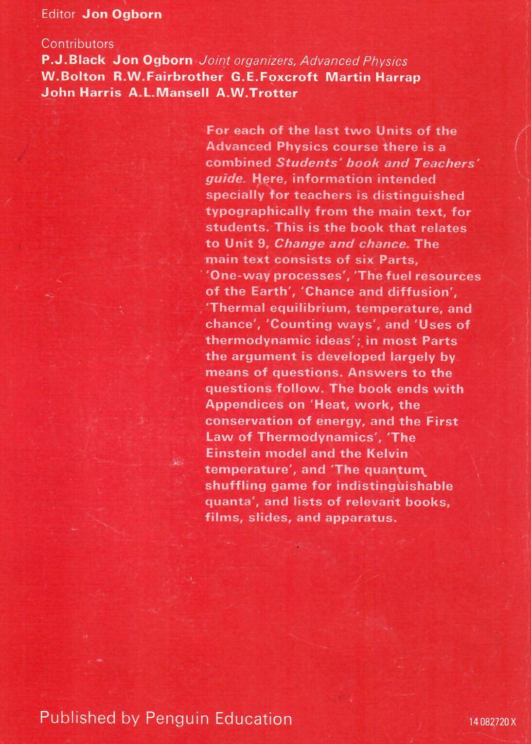
Q2 The sketches in figures 1 to 4 show instants from sequences of events. The times between instants in a, b, c, and e are all equal. Some sequences have been printed in reverse order. Decide whether each sequence is in the normal order or is in reverse order, or explain why you cannot tell.
a An oscillating simple pendulum.
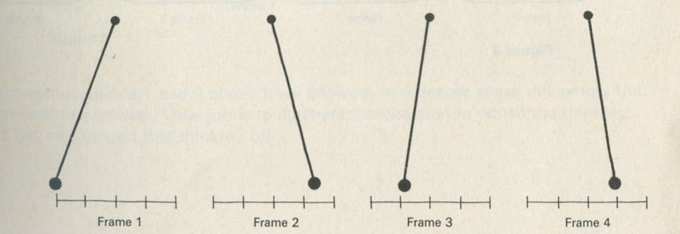
Figure 1
Full Size Image
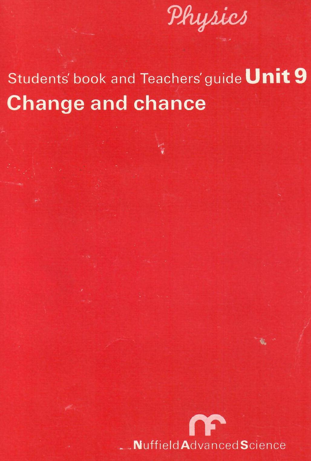
b Marbles being shaken in a container. The marbles are of two different colours, but they are otherwise identical.
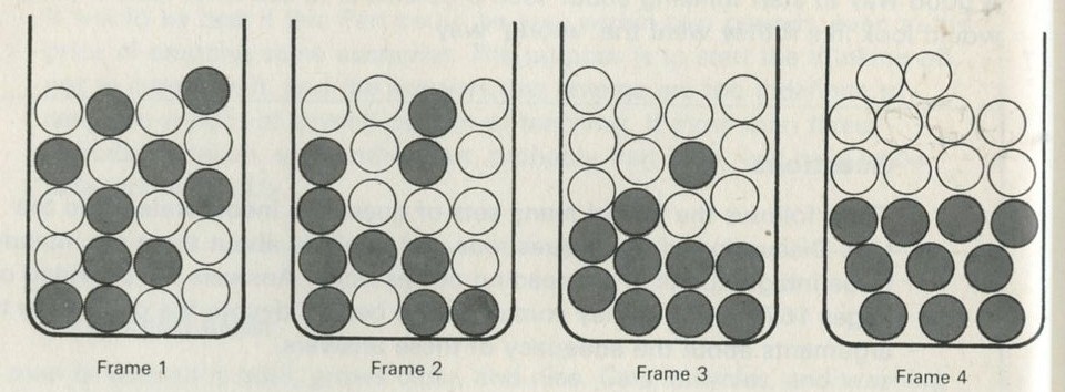
Figure 2
Full Size Image
c Same as b but there are only two of each sort of marble.
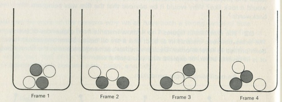
Figure 3
Full Size Image
d Two beakers of water in thermal contact.
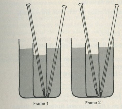
Figure 4
e A ball rolling on a horizontal table.
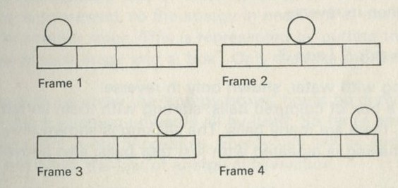
Figure 5
Although questions 1 and 2 above have answers, in a deeper sense this whole Unit provides their answer. Their job is to illustrate the direction in which the thinking will go, and to start that thinking off.
Film loops, Forwards or backwards?
Three 8 mm loop films, specially made for this Unit, are available. See the film list for details.
Forwards or backwards? Loop 1
- Event A: A brick falling to the floor, shown first forwards and then in reverse.
- Event B: A piece of red hot steel being dipped into water, shown first forwards, and then in reverse.
- Event C: A piece of paper burning, shown first in reverse, and then forwards.
Forwards or backwards? Loop 2
- Event A: A ball bouncing on a flat, horizontal surface, first shown forwards and then in reverse.
- Event B: A vehicle travelling to and fro along an air track, shown only in reverse.
- Event C: A collision between a pair of nearly frictionless pucks, shown first forwards and then in reverse.
Forwards or backwards? Loop 3
- Event A: Ink mixing with water, shown only in reverse.
- Event B: Shaking a box of coloured balls, starting with them sorted into two layers. Initially, there are many balls. The shaking is shown only in reverse. Then the shaking is repeated with just four balls, also shown only in reverse.
- Event C: The film shows a row of heavy pendula, which are not coupled but have various lengths. First, just one pendulum is shown swinging on its own, in reverse only. Then uncoupled pendula of various lengths, in a row, are shown swinging together, both forwards and in reverse.
The purpose of these films is to focus attention, through discussion, on the problem of why some events look absurd in reverse while others look sensible. In Part Two the implications of the special case of the one-way burning of fuels are considered.
Energy changes
What energy transformations occur when a brick falls from a height onto the floor? Initially, the brick has gravitational potential energy. As it falls this energy is transformed to kinetic energy of the brick. When the brick hits the floor this energy passes to extra energy shared among the molecules of the brick and the floor - the temperatures of the brick and of part of the floor increase. The energy transfer of gravitational potential energy to energy shared among molecules is quite sensible - bricks often fall. The reverse event, with the brick jumping up off the floor, does not seem sensible.
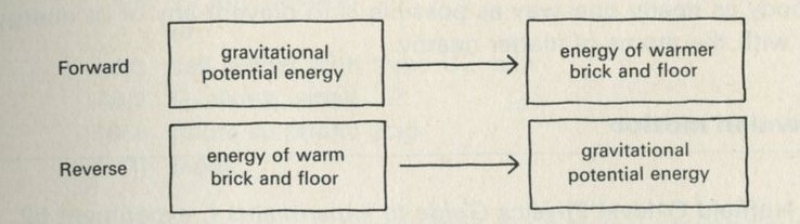
Figure 6: Energy boxes showing energy transfers
Full Size Image
Figure 6 suggests a way of drawing a diagram to represent energy transformations. Energy is conserved, so the energy in one form at one stage will appear in another form at another stage. This is represented by putting the name of the form of the energy at each stage into a box. Only the first and last stages are shown.
Figure 6 shows how the energy boxes could be drawn for the impossible event of the brick jumping upwards all by itself. So far as energy is concerned, this reverse event is not impossible. Energy can still be conserved; the reverse process does not break the law of energy conservation.
The First Law of Thermodynamics
Appendix A discusses the difference between the First Law of Thermodynamics and the Law of Conservation of Energy.
The Law of Conservation of Energy is thus no help in determining the direction of an event. The law would allow a hot brick and the floor to cool, and so to provide the energy for the brick to leap into the air. For this to happen the molecules would have to move in unison, so that they all hit the brick at the right moment, and lose energy as they push it into the air. As bricks do not generally leap off floors, such organized movement must be very rare. It does not appear likely that the molecules will move in just the right way to hit the brick upwards.
Q3 Draw energy boxes for a a piece of paper burning, b an air track vehicle travelling forwards and backwards along a horizontal track.
Q4The piece of paper burning does not look sensible when reversed; the vehicle moving along the air track does look sensible. Do your answers to question 3 give any clue to why one event looks sensible when reversed and the other does not?
If there is one word which is the key to the difference between one-way and two-way processes, it is spreading. Whenever motion or energy becomes spread out among many particles, something two-way has happened. The trick for making the motion of a body as nearly one-way as possible is to prevent any of its energy from being shared with the atoms of matter nearby.
Brownian motion
See Nuffield O-level Physics Guide to experiments I, experiment 52. Any student who has not seen Brownian motion should see it now.
In the Brownian motion experiment smoke particles are seen being knocked around as a result of gas molecules hitting them. Some of the kinetic energy of the gas molecules has been given to the smoke particles. This is similar to the hot brick and floor getting cooler and the brick jumping up from the floor; a sufficient number of gas molecules have moved together to hit the smoke particle (in one direction) at the right moment, lose energy, and give the particle a push. There is, however, one significant difference between the smoke particle and the brick - the smoke particle is considerably smaller. Not so many molecules have, by chance, to hit it in unison in order to produce an observable motion.
Q5 Which is more likely, that everyone in a class of only three students might choose by chance to go to the cinema at the same time, or that everyone in a class of forty students might choose to do so, again by chance?
Q6 Would a film of Brownian motion look sensible if run in reverse?
A process in which energy is shared out among many molecules looks implausible in reverse. The sharing must be among only a few molecules to be plausible in reverse. Two-way processes usually involve large numbers of objects.
9.1 Demonstration: Energy conversions
  9A   motor/generator unit
  9C   switch unit
  9D   lamp unit
  9E   flywheel unit
  9L   storage battery unit
  9M   driving belt
 176   12 volt battery
       or
1033   cell holder with three U2 cells
44/2   G-clamp, small   2
1056   dilute sulphuric acid
1000   leads
a A motor driving a flywheel; then the flywheel driving the motor as a dynamo.
See Nuffield O-level Physics Guide to experiments II, experiment 61 (21).
b A pair of lead plates dipping in sulphuric acid charged from a battery, then used to light a lamp.
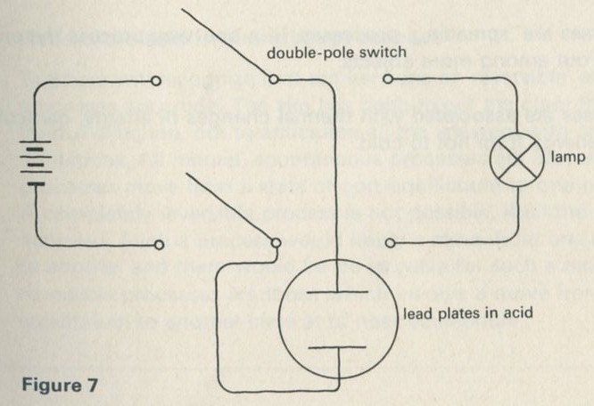
Figure 7
Full Size Image
The storage battery unit, filled with dilute sulphuric acid, is connected via the switch to the battery (4 or 4.5 V) and to the lamp unit (using one lamp only). When the switch is thrown over to connect the lead plates to the lamp, the lamp will light for a few seconds.
One-way and two-way machines
Some machines are used to change energy from one form to another. The transformation could be of electrical energy to mechanical energy, or of mechanical energy to electrical energy, for example. Films of some machines would look sensible in reverse.
Q7 Suggest a machine which, if shown running in reverse on a film, would still look reasonably sensible.
Q8 Draw energy boxes for a lead-acid battery driving a motor which lifts a load. Could this process work backwards?
Q8 Draw energy boxes for a lead-acid battery lighting a lamp. Could this process work backwards?
Clearly, the distinction between one-way and two-way processes is a matter of practical importance, and is not merely an intellectual puzzle.
Summary: What kinds of events are one-way?
The Law of Conservation of Energy is no help - every change it allows one way it allows the other.
One-way processes are spreading processes. In a one-way process the energy becomes spread out among more objects.
One-way processes are associated with thermal changes of energy, particularly the thermal flow of energy from hot to cold.
Mixing processes
In Part Three, we look at mixing, jumbling, and diffusion as other examples of one-way processes. If students raise such ideas now, the teacher may want to use material which occurs at the beginning of Part Three.
Difficulty over the meaning of one-way processes
There may be a difficulty over the meaning of one-way processes. As they have been described, the melting of a lump of ice is one-way, but students may object that the water can, after all, be frozen again. To freeze it, a cooling device is needed, driven by some source of energy. Perhaps the energy is electrical, from a hydro-electric power station; then some water ends up at the bottom of a hill instead of being at the top. How might it get back? The Sun could evaporate it, and it could then fall as rain, having spread the energy liberated on condensation out into the atmosphere. So the water can be frozen again, but not without other one-way processes going on. It is not possible to go back to the starting point with everything in the world exactly as it was before. Bent's The Second Law, Chapter 4, discusses this problem.
Reversible and irreversible processes
Teachers will recognize that our versions of reversible and irreversible processes are crude. The aim has been to get the class thinking in a fruitful direction, not to anticipate all the answers with careful definitions. All natural, spontaneous processes are irreversible. Such processes move from a state of non-equilibrium to one of equilibrium. A completely reversible process is not possible, if all the side effects are included. Such a process would imply a move from one equilibrium state to another and there would be no impetus for such a move. Nearly reversible processes are those which involve a move from a state near to equilibrium to another state at or near equilibrium.
2. The fuel resources of the Earth
That which burns never returns
(A slogan seen on the vans of a fire appliance company)
Timing
No more than a double period can be afforded for this Part, unless sacrifices are made elsewhere.
World consumption of energy
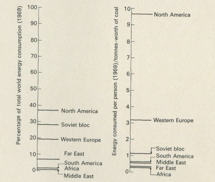
The United Nations statistical yearbook (1965) says that in 1964 the world as a whole consumed energy from fuels equivalent to the energy obtainable by burning nearly 5000 million tonnes of coal. (1 tonne is 1000 kg, very nearly 1 ton.) As there were about 3000 million of us, each person's share was the equivalent of about 1500 kg of coal; that is, about 1.5 tonnes-worth each. But of course the shares were not very even. North Americans consumed about 8.6 tonnes-worth each, and the United States with 6 per cent of the world's population consumed over 30 per cent of the total energy. Western Europeans consumed nearly 3 tonnes-worth each, while the inhabitants of the Far East and Africa consumed one-tenth as much each, equivalent to 0.3 tonne.
Figures 8 and 9
Full Size Image
From Statistical Office (1969) Statistical yearbook. United Nations.
This uneven distribution of energy use among areas of the world is not simply a matter of unfair shares. A country cannot use energy if it has few power stations or industries to make fuel-using devices, and the Middle East offers a clear example of the difference between having and using energy. It produced 568 million tonnes-worth, but used only 53 million, so that each person consumed about the same as anyone else in Africa and Asia, that is, the equivalent of about 0.34 tonne each.
The richer countries do help the poorer ones with aid, the total flow of international aid from all sources being estimated for 1960 at about 2.9 thousand million dollars. In 1952, the United Nations report, Measures for the economic development of underdeveloped countries, estimated the need for aid to be about 20 thousand million dollars a year. The largest single contribution to economic aid comes from the United States. The survey (1964) of the U.S. economy, by the Organization for Economic Cooperation and Development, quotes 725 million dollars for government grants and capital in the form of dollar payments abroad for 1964.
The energy figures should suggest at least two questions. How is energy consumption connected with the degree of industrialization, or advancement of a society? What prospects can we see ahead as more and more people want, for example, to have cars which use up petrol, and are made of steel which is costly in fuel to extract and manufacture? Secondly, how big a dent was made in 1964 in the world's stock of coal, oil, gas, and other energy sources as yet untapped?
We shall now consider the second question in detail. The equivalent of a million tonnes of coal represents a large amount of energy. It comes to 2.8 � 1016 joules. As was mentioned earlier, in 1964 the world as a whole consumed energy from fuels equivalent to nearly 5000 million tonnes of coal. This is 0.14 � 1021 joules or 0.14 Q, where Q ≈ 1021 joules and is a unit that has been used in calculations of world energy resources.
So in 1964, mankind used 0.14 Q. Table 1 gives some figures for the total reserves of fossil fuels left in the earth at the mid-twentieth century.
                       Reserves known to       Additional
                       exist, which            resources whose
                       can be extracted        extraction may
                       using present           or may not
                       methods under           be technically
                       current economic        and economically
                       conditions              feasible
coal and peat            24.7 Q                 53.6 Q
oils                      2.0 Q                 27.7 Q
natural gas               0.7 Q                  7.6 Q
oil shale and tar sands   0                     13.1 Q

Total                    27.4 Q                102.0 Q
(Q = 1021 J)
Table 1: Reserves of fossil fuels
Data from Statistical Office (1965) Statistical yearbook. United Nations
Q1 If the world were to go on using energy at 0.14 Q per year, how long would the reserves that we know can be extracted last (assuming that only fossil fuels are used)?
As the reserves that we know can be extracted run out, no doubt men will find ways of tapping some of the 102 units of additional resources. But will the world go on consuming energy at the 1964 rate?
Figures 10
Full Size Image
From Putnam, P. C. (1954) Energy in the future, Van Nostrand Reinhold Co.
Figures 11
Full Size Image
From Putnam, P. C. (1954) Energy in the future, Van Nostrand Reinhold Co.
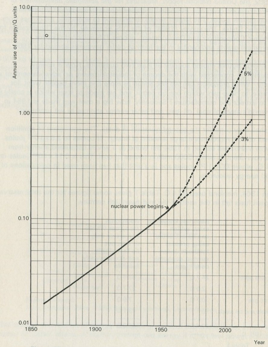
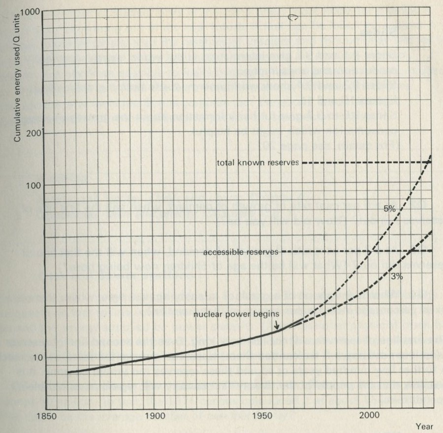
Figure 10 shows what has happened in the past, with some guesses about the future, based on the growth of population and the rise in the energy demands of each individual. Back in 1850, the world was spending about 0.01 Q per year; by 1950, this was about 0.1 Q (as we have just seen). Figure 11 shows the cumulative use of energy. In the 2000 years up to 1850, man is thought to have burned between 6 and 9 Q. By 1950, the world had burned nearly twice as much, about 13 Q, so that the century from 1850 to 1950 was nearly as expensive as the previous twenty centuries. Both graphs show what will happen if energy consumption per person increases at 3 per cent and also at 5 per cent per year. These are limits, based on the likely increase of population and industrialization, within which it is anticipated the increase will occur. Over the period 1931 to 1950 the rate of increase was 3 per cent, an increase over the previous period. The rate of increase was, however, far greater for industrialized nations.
Slides
Slides 9.1 and 9.2 give information about world energy reserves, production and consumption.
Slides 9.3 and 9.4 show world energy consumption graphically as in figures 10 and 11.
Slides 9.5 to 9.7 give further information about the growth of energy consumption which might be helpful.
(For details, see the slide list.)
Q2 At a 5 per cent rate of growth of demand, when will the first line of reserves run out? (How old will you be?)
Q3 At a 3 per cent rate of growth of demand, when will the first line of reserves run out? (What will be the age of children now being born?)
Q4 What is the shape of a graph of quantity against time, where there is a fixed percentage increase per annum in that quantity?
The first line of reserves will not last very long. Even the second line of reserves (and it is not known if we can tap them) does not improve the picture very much. A further few hundred years or so and these reserves too would be gone. It is possible that the people of the twenty-first century will regard us as terrible spendthrifts.
Why worry - energy is conserved?
Why should we worry about running out of fuels? Energy cannot be lost; it has merely been transferred from natural gas, coal, or oil, and oxygen, to warm the atmosphere. Why can we not use this energy, assuming we could trap it? There is a link here with Part One: burning was definitely one of the one-way processes. When fuel is burned, something irreversible has been done. Having done it, one can never go back.
Energy resources other than fossil fuels
The Sun delivers about 3000 Q every year to the surface of the Earth, but the energy is very much spread out, being roughly a few hundred watts to each square metre.
This flow of energy can be tapped without using up the store of fuel. The main way of using it is by hydro-electric power generation, but at present this source only provides about 1 per cent of world consumption. It is hard to imagine hydroelectric power being expanded enough to take over from other sources.
The available stock of nuclear fuels in the Earth offers more hope, for a while at least, of our not running out in the near future. If fuel can be bred in reactors from low grade materials, then the reserves of uranium and thorium may last for a long time. The disposal of the radioactive wastes will be a severe problem, however. If it becomes possible to make hydrogen fuse into helium in a controlled way - the reaction that fuels the Sun - then the energy future looks brighter. (The reaction that fuels the Sun is complex, but the above is its net effect. Proposed earthbound reactions involve the use of isotopes of hydrogen.)
Reading
Angrist and Hepler, Order and chaos, Chapter 4.
Ubbelohde, Man and energy, Chapters 4, 5, 7.
Cars and power stations
The motor car is one symbol of industrial society, and it is a great user of energy. The questions that follow invite you to make guesses about the energy used by cars and the energy supplied by power stations. (A professional physicist often has to make rough guesses. It is part of his scientific skill to make those guesses as well as he can, and also to have some idea of how good or bad the guesses may be.)
Q5 Guess how many cars there are in Great Britain. Assume that the population is about 50 million (in fact, the 1971 census calculated it at about 55� million). What might be the average number of cars per family?
Q6 Guess how much total power there is installed in these cars. (One horsepower is three-quarters of a kilowatt.)
Q7 Guess how much power is installed in power stations in Great Britain. Will it be more or less than the car-power?
Q8 Guess how much petrol the cars would use in a year. How much energy is involved?
(One gallon of petrol is about 4 kg. One tonne of petrol is equivalent to 1.7 tonnes of coal. One tonne of coal is equivalent to 2.8 � 1010 joules.)
How well was this energy used? The energy accounts for cars suggest that they are rather wasteful. Typical figures are given in table 2 below.
Process using energy                       Percentage used

wind resistance                             10
                                                    20
road friction                               10

transmission, generator, fan, pumps, etc.    5       5
radiator and engine heat losses             35
                                                    75
exhaust, oil, and other losses              40
Table 2
Use of energy by a car driven at a steady speed, say 80 kilometres per hour.
From Burke et al. (1957) Trans. SAE, 65, page 715.
Only about 20 per cent of the power of a car's engine is used to move the car along. Three-quarters of the fuel energy goes directly to heat up the atmosphere. The study of heat and molecules will show, remarkably enough, that this regrettable state of affairs is not due to incompetence on the part of designers of engines. We shall see that it is inevitable that some heat is thrown away. See Inefficient engines.
Power stations also throw heat away; indeed most people recognize power stations by their vast cooling towers. (Figure 12.)
Q9 Figure 13 shows a power station with no cooling towers. How does this power station get rid of its exhaust heat?
Fortunately, power stations are more efficient than cars, and the best of them onvert nearly 40 per cent of the fuel energy to electrical energy. In 1925, the figure for an average power station was nearer 20 per cent. Possible further improvement in the efficiency of power generation is one important reason why people are interested in thermodynamics.
Q10 A question to think about. What might be some of the effects on the environment, and on the world as a whole, of the exhaust heat of the power stations needed to cope with the energy demand?
Slides
Slide 9.9 shows the growth in the number of cars in Britain.
Slide 9.10 presents the data on the energy account for a car.
Slides 9.11 and 9.12 show the power stations also shown in figures 12 and 13.
Supplementary material
This concludes the work we suggest for this Part. The extra suggestions that follow are intended for those who can find extra time and who wish to follow up an interest.
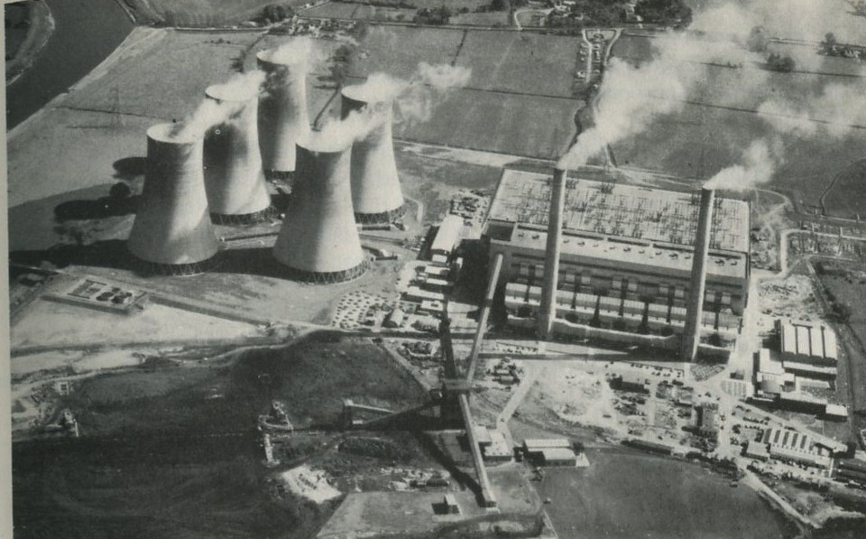
Figures 12: A power station, with cooling towers (High Marnham). Photograph, Central Electricity Generating Board.
Full Size Image
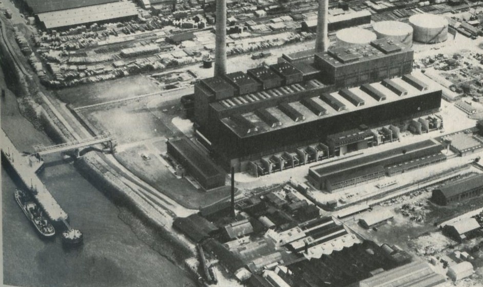
Figures 13: A power station, without cooling towers (Belvedere). Photograph, Central Electricity Generating Board.
Full Size Image
How men create energy
In primitive societies, most men can just grow enough food to feed themselves, and gather enough fuel to warm themselves. There is little left over from their basic needs for other purposes.
The beginning of coal mining made an important change in this situation. The energy available from burning the coal mined by one man was some 500 times larger than the food-energy needed to keep that miner healthy and working. The coal could then be used in engines to do more work; each man-day of a miner's effort created the equivalent of several more man-days of work which could not otherwise have been obtained.
This may sound desirable, but it has some social consequences that are being felt more and more. All that unskilled labour can offer is energy, and alternative sources of cheap energy leave the unskilled with little to offer in competition.
Q11 Guess how much work-energy a man can produce in a working day.
Q12 How much would an Electricity Board charge for supplying as much energy as the work-energy produced by a man in a day?
Q13 What would be some of the social consequences of always using the cheapest source of energy?
Reading
Angrist and Hepler, Order and chaos, pages 79-83.
Ubbelohde, Man and energy, pages 88-93.
Feeding the world
The conservation of energy makes no exception for men. Just to stay alive and warm, a person needs perhaps 5 � 106 J of food-fuel every day. More is needed if he is to be able to do any work, or even just to be able to move around; say 107 J every day. This food-fuel has to be grown, and its energy comes ultimately from the Sun, which delivers about 6 � 1022 J, or 60 Q, to the top of the atmosphere every day. Not all the energy reaching the top of the atmosphere reaches the Earth's surface: the amount that does so is about 30 Q every day. Less than half of this energy, say 10 Q, is available for photosynthesis. The present plant populations on land and at sea use about 1/5000 of this energy in photosynthesis, because they cannot possibly catch and use it all. So the Earth can produce roughly 2 � 1018 J (2 � 10-3 Q) edible joules per day.
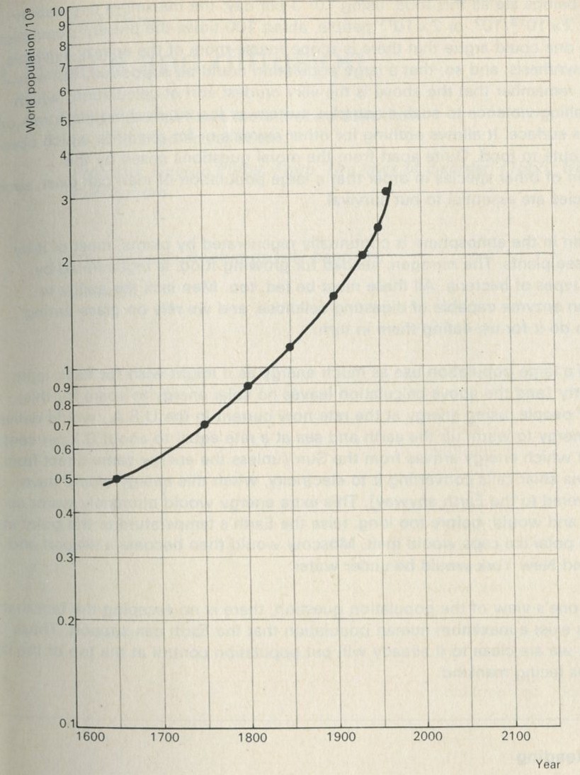
Figures 14
Full Size Image
Data from Thomson, W. S., 5th revised edition (1965) Population problems, McGraw-Hill.
If human beings ate all this food, using 107 J per day, the maximum population would be 2 � 1018/107, or 2 � 1011 people, about 100 times the present population. Certainly, one could argue that there is scope to use more of the energy available for photosynthesis, and so, that a large population could be supported. But one must also remember that the above is the very crudest sort of calculation, which does appalling violence to such a complex system as the interlocking life forms on the Earth's surface. It allows nothing for other animals or for plant life which does not contribute to food. Quite apart from the moral questions raised by the destruction of other species in order that a large population of men can exist, such other species are essential to our survival.
The oxygen in the atmosphere is continually regenerated by plants, most of it by primitive sea plants. The nitrogen, needed for growing food, is regenerated by chains of types of bacteria. All these must be fed, too. Men lack the ability to produce an enzyme capable of digesting cellulose, and we rely on grass-eating animals to do it for us, eating them in turn.
Nor could a large population use as much energy as it might wish for heat, light, and industry (and the above calculation leaves no solar energy to spare for this). Only 1010 people, using energy at the rate now current in the U.S.A., would deliver enough energy to warm up the earth and sea at a rate equal to about 0.1 per cent of the rate at which energy arrives from the Sun (unless the energy came direct from the Sun, via solar cells converting it to electricity, when this energy would have been delivered to the Earth anyway). This extra energy would ultimately warm up the Earth, and would, before too long, raise the Earth's temperature to the point at which the polar ice caps would melt, Moscow would then become a seaport and London and New York would be under water.
Whatever one's view of the population question, there is no escaping the fact that there does exist a maximum human population that the Earth can support. Those who think we are close to it already will put population control at the top of the list of priorities facing mankind.
Reading
Angrist and Hepler, Order and chaos, Chapter 6.
3. Chance and diffusion
'There are few laws more precise than those
of perfect molecular chaos.'
Professor George Porter. From 'The laws of disorder' (1965) BBC Publications.
'The probable is what usually happens.'
Aristotle.
Timing
In this Part, simple quantitative ideas about counting numbers of ways are introduced. With experts, the matter could be disposed of in half an hour. The difficulty for a student is not that the calculations are hard, but that what is going on and why it is being done are not obvious, and that time is needed to learn a new style of thinking.
Some students, especially those who have met the ideas elsewhere, will need little time. Others will need more, but the substance of Part Three is too slight to support more than about half a dozen lessons. It should be remembered that this Part serves to introduce ideas which will be used, and so revised, in later Parts.
The purpose of the discussion about chance and diffusion
This Part is, to some extent, a digression from our main theme, which is an understanding of the flow of heat and thermal equilibrium. Its purpose is to prepare the way for that understanding, which will come out of questions about the random sharing of energy amongst atoms. These matters, discussed in Parts Four and Five, are quite subtle, though they are far-reaching in their consequences.
In Part Three, therefore, we look at how similar ideas can be applied to a simpler, if less important problem: the mixing of one substance with another. The results of Part Three are not, however, all trivial. Most chemical reactions involve the mixing of substances, and this fact has direct consequences for the way the progress of a reaction depends upon the proportions in which each substance is present. Some of these consequences are drawn out in Part Six, which deals with applications of the ideas developed in the rest of the Unit.
In Part Three, we also introduce one other idea we shall use later. This is the notion of using dice-throwing games to imitate some features of the behaviour of systems which are subject to chance. This tactic makes it possible to find out how a system behaves by a mathematical experiment, so reducing the need for mathematical calculations.
Diffusion and mixing as one-way processes
As in Part One, there is something to be learned about the one-way nature of some processes by watching films of events, run backwards. While studying Part One, you may have seen the filmed episodes which we shall now discuss in some detail.
Film loop
Forwards or backwards? 3, is the loop which is appropriate here. The three events it shows are summarized in Film Loops.
Most mornings, the writer, while helping to get breakfast ready, pours hot milk into a jug which has been heated by having had hot water in it. On occasional bad days, he forgets to pour away the hot water before putting the milk in the jug. No doubt the feeling of tragic helplessness this always produces in him is partly the consequence of his half-awake early-morning state of mind, but it also owes something to the impossibility of undoing what has been done, in any simple way. The mixing of milk and water happens all on its own, without any assistance or encouragement, but unmixing them is a different matter altogether.
A film of the mixing of ink and water, shown in reverse, reinforces the point by the very absurdity of what one seems to see. The question is why such spontaneous unmixing looks absurd. Why is it one of those things which never happen? Although it is not at all hard to say more or less why spontaneous unmixing of this kind does not happen, or is at least most unlikely, it turns out that a good, clear account of this rather trivial matter can be used to help in the discussion of much harder matters, like the flow of heat. So it is worth pursuing a little further.
Spontaneous unmixing which does happen
Silt does separate from muddy water, and cream does rise to the top of a milk bottle. The unmixing of the two lots of balls in Event B in the film loop described above would not be absurd if one lot of balls were denser than the other. Such issues may need to be dealt with if they arise. Notice first that none of them would happen in a spacecraft, free of gravitational fields (or the imitation field produced by centrifuging). The falling silt particles, or the rising (low density) fat globules in cream, both transfer energy from gravitational potential energy to (ultimately) energy shared among all the atoms and molecules in the system. The water or milk becomes a shade warmer as the separation occurs. The separation does occur if the increase in the number of ways of arranging, among many molecules, the extra internal energy not now stored as potential energy, outweighs as a factor the decrease in the number of ways of rearranging the silt or fat particles if unmixing takes place.
A collection of many two-way processes can look one-way
A swinging pendulum with a massive bob, hung from a stout beam, is about as near as one can easily get in a school laboratory to a process which looks just as good if it is shown as a backwards-running film, as it does if the film goes forwards. Apart from a little damping, the pendulum's energy is not spread around amongst the molecules of nearby material, and its motion is nearly two-way.
A row of such pendula can be hung in a line. If they are not connected together, and the beam from which they hang is rigid, no one pendulum affects any other, and each one continues its undisturbed two-way motion if it is set swinging. Now suppose one saw such a row made of pendula of different lengths, swinging in no special relationship to one another. Then suppose that as one watched, all the pendula gradually began to come together, and all at one moment rose exactly together to their greatest height on one side. If one wasn't dreaming, the only way it could have been achieved deliberately, would be for someone to have worked it all out in advance, and then set each pendulum swinging with just the right motion so that, in the end, as all the swings changed their relationships to one another, the pendula swung together for a moment.
To achieve all this would have been a considerable feat of ingenuity. As you may have seen, another way to make it seem to happen is to start the pendula off together, film their motion, and then show the film backwards. To an excellent degree of accuracy, no one pendulum motion seen on the reversed film is impossible: the motion of a pendulum which is not damped is just as possible either way round. But the collection of many motions, everyone of which is two-way by itself, looks decidedly one-way. The effect solely depends on large numbers.
The effect is not one to puzzle over unduly, though it is worth seeing, if only for its visual charm. If one wants to, one can find some quite deep puzzles in it, which have concerned a number of physicists and mathematicians. For example, wouldn't the pendula come together if one waited long enough? Can a large number of truly reversible processes really add up to something irreversible, or is this just an effect of what one expects to see, not of what one ought to expect? But none of these are puzzles you need follow up now, unless you want to.
Large numbers and small numbers
The particular aspect of mixing which we shall follow up is that aspect which does not involve energy in any way, but simply the muddling together or sorting out of particles among one another, or the spreading out of particles into unoccupied spaces. A simple system which illustrates this aspect is a box containing two sorts of coloured balls. The balls differ only in having one colour or the other, and in no other way. If the box is shaken after the balls have been sorted so that those of each colour are together, everyone knows what to expect. The balls become mixed, and the process seen in reverse looks very strange; no less strange than the act of a conjurer who shuffles a pack of cards and ends up with them in perfect sequence.
What is interesting and illuminating is to see the same shaking process when there are only a few balls in the box, say two of each colour. The constant interchange amongst the balls now looks just as reasonable in reverse as it does in the real life direction. The mixing of many balls is a one-way process, but the mixing of just a few is not. The number of objects involved is an important factor in deciding whether a process is one-way or not.
Q1 When a box containing many marbles of two colours is shaken, is the reason why they do not sort themselves out that they cannot do so?
Q2 Shaking the box containing many marbles rearranges the marbles among each other, going from one way of arranging them to another, and to another. Would you say that there is just one way, or that there are a few ways, or that there are many ways of rearranging them, such that you would say that the marbles were well mixed?
Q3 There is at least one and perhaps there are many possible ways of arranging the marbles so that anyone would agree that they were pretty well sorted out into the two colours. Would you say there were more than, fewer than, or the same number of ways of doing this as of achieving arrangements which one would naturally call muddled or well mixed?
If just four marbles are shaken so as to stay in a two-by-two array, but so as to interchange places, all the possible ways of arranging them can be set down, as in figure 15 (ignoring interchanges of similarly coloured marbles).
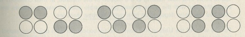
Figure 15: Patterns of arrangement of four marbles, having two colours.
Full Size Image
One could say, of the two ways shown on the left in figure 15, and of only these two, that the marbles are vertically sorted. If you shook the marbles and then inspected them, they would have to be arranged in one of the ways shown. Suppose that the marbles are smooth and round, and that nothing favours one way of arranging them over another.
Q4 If they start off in one of the vertically sorted ways, and are shaken, could they ever, by chance, end up again in one of the vertically sorted ways?
Q5 If you shook them, and inspected them a great many times, about how often might you expect to see them vertically sorted?
Q6 Why, in question 5, would you not expect to see them vertically sorted quite as often as in some other pattern?
Chance is enough to work out what happens on average
In discussing the interchanges of four marbles (questions 4 to 6) we almost casually introduced the idea that one might reasonably suppose that nothing would favour any one of the ways of arranging the marbles (shown in figure 15) over any other way. We now propose to take this idea more seriously: indeed it is the key to understanding the work of the whole Unit.
Optional experiment: 9.2 Random motion of marbles in a tray
Much can be learned from watching marbles rolling about at random in a shallow tray. If for any reason you have not done so before, you would be well advised to spend some time now looking at the motion of the marbles, at their collisions with each other and with the walls, at how far a marble goes between collisions, and at how this last point depends on how many marbles there are.
For the work of the Unit, at this point, we are concerned with one other aspect. Imagine the tray to be divided into two halves, or draw a line across its middle, and look to see what proportion of the marbles is, on average, to be found in any one half. Look also to see how far the number in one half seems likely to deviate from the average number.
Optional experiment: 9.2 Random motion of marbles in a tray
    12     two-dimensional kinetic model kit
 optional extras:
   133     camera
   171     photographic accessories kit
  1054     film, monobath combined developer-fixer
           slide projector
Shake the tray with about ten marbles in it, keeping the tray level. There should be a line drawn across the middle of the tray, dividing it in half, drawn on a sheet of paper laid in the tray if it is desired not to mark the cork mat.
If it will be of interest, photographs like those in figures 101a and 101b, Appendix D, can be taken. The camera may need an auxiliary lens (figure 16), the lens being held with the tray at its principal focus and the camera being focused at infinity. The tray can be shaken by hand or with more trouble, by a crank driven from a motor. Good results have also been obtained with a Perspex plate, and 1 to 2 mm ball bearings contained within a wall made of a second sheet of Perspex with a rectangular hole cut in it, as in figure 17. The wall is driven at 50 Hz by a vibrator. This device can be fitted on an overhead projector.
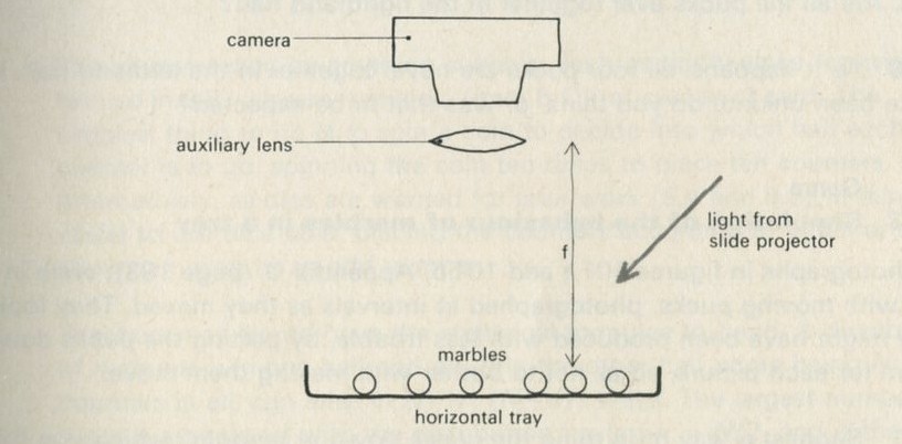
Figure 16: Photographing balls rolling in a tray.
Full Size Image
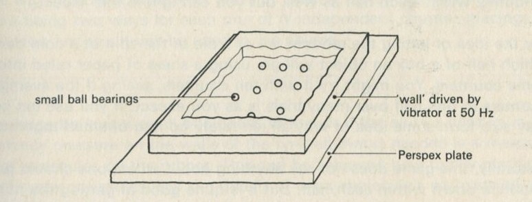
Figure 17: Alternative ball-rolling apparatus.
Full Size Image
You may, however, feel that you have rolled marbles in trays often enough before. If so, you may prefer to look at the photographs of pucks moving on an almost frictionless surface, reproduced in figures 101 a and b, Appendix D.
Q7 In figure 101 a, a series of snapshots of ten pucks moving about on a horizontal surface is seen. Are all the pucks ever together in the righthand half?
Q8 What is the average number of pucks on the righthand side? Is it what you expect? (There is a quick way to find the average. Guess the answer, then score 0, + 1, + 2, -1, etc. for each frame, according to whether the number in one half is different from your guess. The average is found from the total of these scores, many of which cancel as you go along, divided by the number of frames, and added to your guessed answer. The better your guess, the easier it is.)
Q9 In figure 101 b, there is a similar set of photographs, but with only four pucks. Are all the pucks ever together in the righthand half?
Q10 As it happens, all four pucks are never together in the lefthand half. Has chance been unkind, do you think, or was that to be expected?
Game: 9.3 Simulation of the behaviour of marbles in a tray
The photographs in figures 101 a and 101 b, Appendix D , were in fact taken with moving pucks, photographed at intervals as they moved. They look as if they might have been produced with less trouble, by putting the pucks down at random for each picture, so as not to bother with making them move.
Q11 Suggest a way of putting the pucks down at random, which you think ought to divide them between the two halves in the same kind of way as they are divided in the pictures. (To imitate the pictures one would have to place the pucks randomly within each half as well, but you can ignore this aspect.)
Try the idea of letting the random fall of a die or the spin of a coin decide into which half of a box an object will go, using a sheet of paper ruled into two, and some counters. You might try it with ten counters, seeing if the average number of counters in one half over many trials is as you expect. If you use ten counters, you may also form some idea of why all ten rarely go into one half together.
Naturally, this game does not say anything about where one should put the counters down within each half. But it is quite good at getting the numbers in each half right. This is typical of random simulation methods: they often predict average behaviour well, without representing or predicting the detailed behaviour of a system at all.
Game: 9.3 Simulation of the behaviour of marbles in a tray
     1053     counter 10
     1054     graph paper
     1055     die or coin
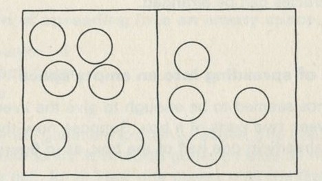
Figure 18
The counters may be anything suitable, such as tiddlywinks (convenient for use in 9.8), square pennies (item 5 C), or pieces of card. The simplest thing to do is to spin a coin to decide into which half each counter is to go, spinning the coin ten times to place ten counters. Alternatively, as dice are wanted for later work (9.4 and 9.8), it may be easier to use dice now, placing the counters according to whether the die shows an even or an odd number.
Teachers may like to have the statistical formulae to hand. A distribution ofn counters in one half and N-n in the other half, there being N counters in all, can arise in N!/n! (N-n)! ways. The largest number of ways is associated with the distribution having n = N/2, and is the most probable distribution. The two distributions which have all the counters in one half are less likely than any other, each arising in only one way. The total number of ways of placing the counters is simply 2N , there being two ways for each one of N independent counter-placings. Only this last result will be used in the course.
Often, the average behaviour is all one needs to know. If the air in a car tyre is to maintain a steady pressure on the walls of the tyre, all that is needed is a reasonably steady hail of molecules on the rubber. This can be achieved by a totally random movement of many molecules, and the details of every molecule's path, speed, and collisions are of no importance.
The first game, 9.3, suggests what the average division of pucks or molecules between two halves of a space might be. The next game, 9.4, suggests how one might simulate some aspects of how a system reaches that more or less steady average behaviour if it starts a long way from the average behaviour. The main point of introducing it is that a later game, 9.8, which is crucial to the whole Unit, uses a similar idea, but it will also help in working out a detailed analysis of how the spreading of particles in a mixing or diffusing process depends on the numbers of ways in which the particles can be arranged.
Game: 9.4 Simulation of spreading into an empty space
In the game 9.3, chance seemed to be enough to give the average behaviour of particles divided between two parts of a box. Suppose now that we agree to start with all the counters already in one half of the box, as in figure 19.
Q 12 Is the distribution which has all counters in one half near to the average behaviour if the counters can go in either half?
The question is, how might one now use a die to move the counters randomly between the halves of the box? If there are six counters, as in figure 19, and each is numbered, a six-sided die can be thrown and the counter whose number comes up can be moved to the half it is not now in.
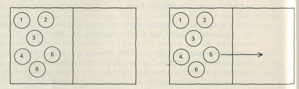
Figure 19
Full Size Image
Q 13 What must happen on the first throw?
Q 14 On the second throw, out of the six possible moves, how many will move a second counter to the initially unoccupied half?
Q 15 On the second throw, how many of the possible moves will take the first counter moved over (counter number five in figure 19) back again to the full half?
Q 16 If everyone in a large class makes two moves, what proportion might end up with all the counters back in the full half?
It is worth going on to make several more moves. Although the die does not know or care when all the counters are in one half, you should find that that distribution arises rather rarely. You should be able to say why it arises infrequently.
Game: 9.4 Simulation of spreading into an empty space
      1053    counter 6
      1054    graph paper
      1055    die
The rules of the game are explained above. The counters need to be numbered one to six. It is worth going on until all the counters happen to go into one half, for at least one player, after the first few moves have spread them between the two halves. After the second move, it is good to take a poll of those whose first-moved counter has gone back into the full half.
Counting numbers of ways
In several discussions in this Part, it has been helpful to think about the number of ways in which a state of affairs can arise. This idea is a crucial one. We shall now use it to calculate one aspect of the behaviour of particles spreading into an unoccupied space. This calculation is the basis of a chemist's thinking about the mixing of reacting molecules. It also serves as an example of a method which we shall put to more important uses in Part Five, in discussing why heat goes from hot to cold, and what hot and cold mean at the level of molecules sharing energy amongst themselves.
One way six counters can be divided between two halves of a box is to have them all in one half. But there are many other ways of arranging them. Suppose there are altogether W ways of arranging the counters between the two halves (including the one way with all in the left and the other one with all in the right).
Q17 Out of many observations, in what fraction of them might you reasonably expect to see all the counters in, say, the lefthand half, in terms of W?
The total number of ways W is easy enough to calculate. Figure 20 shows how to do it. The first counter can be put down in two ways, as in figure 20 a. The second counter can also be put down in two ways, each of which can go with either of the two Ways for the first counter, as in figure 20 b. The third counter can again be put down in two ways, as in figure 20 c.
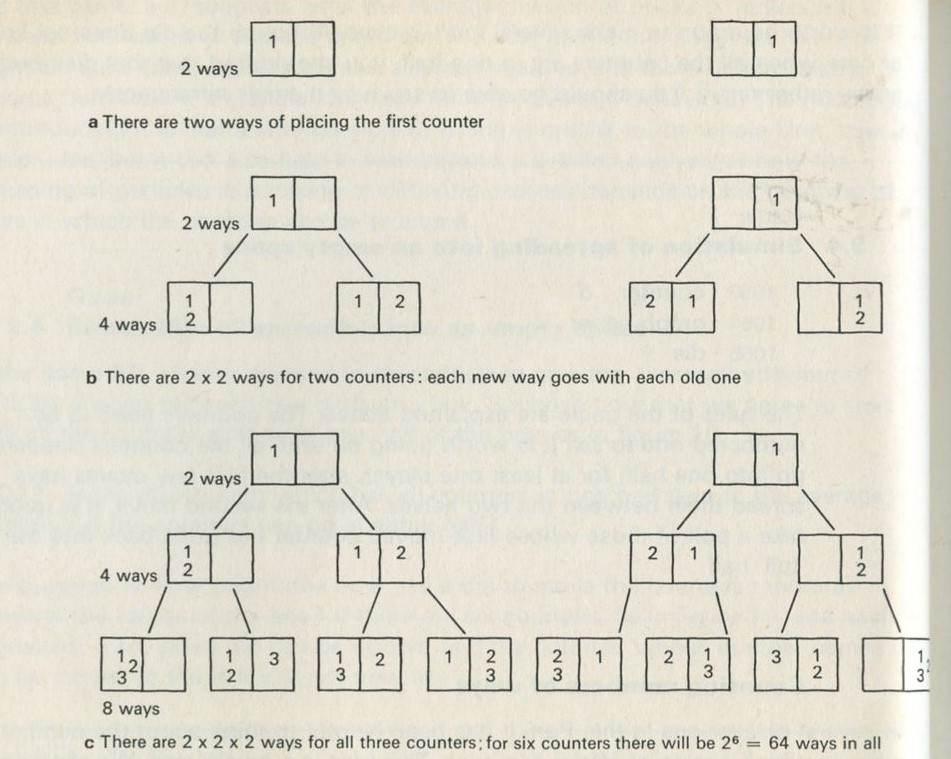
Figure 20: Counting numbers of ways for particles in two halves of a box.
Full Size Image
Each of the two ways for the third counter can go with any one of the previous four ways, giving now 4 � 2 = 8 ways (not 4+2). This last point is of the greatest importance: numbers of ways multiply when they are independent of one another.
If there are four counters, there will be 2 � 2 � 2 � = 24 = 16 ways in all. If there are six, there will be 26 = 64 ways. If there are N counters, there will be a total number of ways given by W= 2N .
Note for teachers
The result W = 2N will be used in Part Six, in a discussion of the entropy change of an expanding gas and, less directly, in a discussion of the effect of concentration on the e.m.f. of a cell. Here, however, its main purpose is to provide an example of the calculation of numbers of ways.
The calculation makes a definite prediction. If N pucks move about at random on a horizontal surface, or if N gas molecules move about in a container, on one observation out of 2N, on average, all N particles may be expected to be in one particular half.
We tried it out using a computer, which was asked to play the game in 9.3 in its head, using four imaginary counters. Instead of spinning a coin, the computer calculated random numbers to decide the fate of each counter. Using N = 4, we expected 1/24 = 1/16 out of a great many trials to end up with all four in one particular half. In 1 minute 11 seconds, the computer made 16 000 trials and 1/16 therefore is just 1000. The outcome is shown in table 3.
Number of counters in the
'lefthand half'              0      1      2      3      4

Number of occasions          1086   3823   6188   3900   1003
Table 3: Results of a computer trial, distributing four counters in two halves of a box.
Optional game: 9.5 Test of calculation of number of ways of arranging four counters
    1053     counter 4
    1054     graph paper
    1055     die or coin
Unless students would think it tedious and unnecessary, there may be value in repeating the game in 9.3 but with four counters, trying it a good many times. This is not too lengthy a business with a large class. The aim would be to see whether, out of many trials, about 1/16 put the four counters all in one half.
An interested student could try to reproduce photographs like those shown in figure 101, though the test may reduce to a statistical method of discovering if the table was level.
If the school has access to computing facilities, the game could also be tried out on a computer, should a student be able to write a programme to do it.
Processes that happen inexorably, but quite by chance
In the game 9.4, with six counters, the counters were more likely to spread into both halves of the box, starting all in one half, than to stay or go back into one half. The larger the number of particles, the smaller is the fraction 1/2N , which indicates the proportion of occasions on which all the particles may concentrate by chance in one half.
Think, for example, of an ordinary gas jar full of air. There will be perhaps 1022 molecules in the jar. (One mole of molecules, N = 6 � 1023 , occupies about 24 dm3 at room temperature. A gas jar might contain 1/50 of a mole.) On less than one occasion in 21022 , all the molecules might by chance be in the bottom half of the jar. The number 21022 is unimaginably large. Its logarithm to base 10 is given by
lg 21022 = 1022 lg 2 ≈ 0.3 � 1022 = 3 � 1021
The number whose logarithm is 3 is 1000, that is, 1 followed by three zeroes.
The number 21022 is 1 followed by 3 � 1021 zeroes. If it were written out, with each zero only 1 mm across, it would stretch a distance 3 � 1021 mm, or 3 � 1018 m. In a year, a flash of light travels nearly 1016 m (a year is just over 3 ≈ 107 s, and the speed of light is 3 ≈ 108 m s-1 ). So the number 21022 would stretch out for 300 light-years, nearly as far as the Pole Star, and more than thirty times as far as the star Sirius.
It follows that the chance of seeing all the molecules in one half is so small as to be negligible, even if one only allows as little as a microsecond for the time needed for molecules to rearrange themselves. (This is not generous, since a molecule takes over a tenth of a millisecond to cross a jar.) See questions 18 to 20. The chance is there, but it is smaller than the chance that all the houses in a country will burn down by accident on the same day, or that all the people in a country will just happen to catch measles. Insurance companies do well enough despite the chance of such disasters, while physicists, chemists, and engineers can rely on chance working the way they expect, so huge are the numbers of molecules involved. It follows that if all the molecules are in one half, but are allowed to pass into the other half, they will do so with all the appearance of inevitability. Diffusion is a one-way process because it is so very, very likely, that in effect it always happens.
Nor should you suppose that very large numbers of particles have to be involved for the chance of reverse diffusion to be negligible.
Q18 Suppose there are only 100 molecules in a jar. Write down the logarithm of the number 2100 as a power of ten.
Q19 Now suppose you look at the jar every microsecond. For how many seconds might you have to wait on average before, by chance, all the 100 molecules were in one half?
Q20 People think the Universe is about 1010 years old, which is about 3 ≈ 1017 s. How many Universe-lifetimes does the answer to question 19 represent?
Everyone is disturbed by these large numbers when they are first encountered. Their very vastness, which so defeats the imagination, is what lies behind the paradox in the previous heading, Processes that happen inexorably, but quite by chance.
Summary
Chance is blind: it tries out everything impartially. Things which can happen in many ways therefore happen often. Molecules which can spread into a larger space will do so. This need not be because they are pushed into the empty space, but can simply be the result of chance. There are more ways of arranging the molecules when they are spread than when they are not, and chance will try out all the ways open to the molecules. When there are many molecules, there are many more ways of being arranged when they can spread, and so they do spread. They are so busy trying out all these ways that only rarely will chance take them back to the original unspread condition. The larger the number of molecules, the less likely is it that chance will soon produce a spontaneous reversal of diffusion.
If chance tries out all ways of arranging molecules impartially, an event which arises in twice as many ways as another will be observed twice as often.
Numbers of ways multiply if the choices are separate ones that do not influence each other.
For teachers: further discussion of numbers of ways
Concepts having to do with randomness and probability are not easy to form, and some students may need a good deal of further discussion of examples to help them. The examples should be simple ones, where the answer to the question, How many ways?, is easy to obtain. The more complicated examples such as runs of coin tossing, or the paradoxes involved in, say, the gambler's ruin problem are likely to confuse more students than they assist. A few suggestions follow, and others are to be found in the Teachers' guide Supplementary mathematics.
How often will a die show a four? (One time in six.) Why? (Because there are five other possibilities or ways for it to come up.)
If you don't know which of three books to do your homework in, how many of the class will choose one book? (One in three.) If each person can write in red or black ink, how many choices has each now? (Six - three multiplied by two.)
Why is your desk (or room) more often untidy than tidy? Tidy means evervthing in its place; untidy means some things in other places. If it is left to chance, only rarely will chance hit on the tidy arrangement, just because there are more untidy ones. So chance or forgetfulness will nearly always make a desk (room) untidy and hardly ever make it tidy. The argument that is often used, that, It is no more effort to put things in their proper place than in the wrong place may (or may not) be true, but it is not entirely relevant. It may even be easier to put things away tidily. But there are so many more untidy ways than tidy ones that chance, given the smallest opportunity, will untidy them again. A moment's forgetfulness, or a breeze through a window, and some things will be in the wrong place. If nothing is done about it, there will soon be a lot of things in wrong places.
Teachers can make a point about numbers of ways, and if they were unscrupulous, could make a handsome profit too. Have three cards, each marked with one cross on each face. One card has two black crosses, one has two red crosses, and one has a cross of each colour. Pull one card out of a hat, and put it face down without looking at the lower face. Suppose the cross showing is red. Say, Obviously this isn't the black-black card, so there is an equal chance that it is the red-red or the red-black one. I will bet you even money that the cross on the other side is the same colour as this one. Even a short run of trials will bring a profit, as the odds are really two to one in favour of crosses of the same colour. By the time the teacher has a substantial (but no doubt notional) profit, the class are usually ready to think out what is wrong.
A nice extra point might be raised. If nothing is in its proper place, is that as untidy as possible? Such a confused state might be worse than chance would usually produce, and one would suspect the interference of a burglar. Chance alone would quite likely, by accident, leave some things in their proper places.
Complete randomness does in fact usually look a bit more orderly than one expects. The following set of random numbers is taken from Lindley, D. V., and Miller, J. C. P. (1953) Cambridge elementary statistical tables, Cambridge University Press. The tables are prepared in such a way that each digit is equally likely to appear.
6 1 0 5 6 6 1 8 7 6 8 2 1 1 1 8 6 1 9
0 9 0 3 6 7 8 5 7 3 2 0 6 3 9 9 5 7 5
Is the sequence 9 0 9 0 plausible? Would there really be a run 1 1 1 at random? Aren't there too many sixes? Should 1 8 and 6 1 occur twice? All the ones are in the first half of the sequence. It is random regularities like these that comfort, but ultimately ruin, the roulette player.
4. Thermal equilibrium, temperature, and chance
Timing
This Part is the key to the whole Unit. For some students, it will also conclude the main work of the Unit, except for a glance at one or two applications from Part Six. The times suggested for earlier Parts have been limited deliberately, so as to allow breathing space for Part Four.
We think it may need about a week and a half, say 9 or 10 periods. It could be taught, without interruptions or questions, in much less, but a good deal of time is likely to be needed for discussion, in which students go back over ideas from earlier Parts, and try to see their application here.
Teachers who think their classes can cope with Part Five would do well to go a little more quickly through Part Four. Discussion which might be slow and diffuse in the context of Part Four can be held over to Part Five, when it should be easier to sharpen the issues for those who can grasp the more theoretical development in Part Five.
An improvement in our knowledge of heat, which has been attained by the use of thermometers, is the more distinct notion we have now than formerly of the distribution of heat among different bodies. Even without the help of thermometers, we can perceive a tendency of heat to diffuse itself from any hotter body to the cooler ones around it, until the heat is distributed among them in such a manner that none of them is disposed to take any more from the rest. The heat is thus brought into a state of equilibrium.
This equilibrium is somewhat curious. [Our emphasis.] We find that, when all mutual action is ended, a thermometer applied to any one of the bodies undergoes the same degree of expansion. Therefore the temperature of them all is the same. No previous acquaintance with the peculiar relation of each body to heat could have assured us of this, and we owe the discovery entirely to the thermometer. We must therefore adopt, as one of the most general laws of heat, the principle that all bodies communicating freely with one another, and exposed to no inequality of external action, acquire the same temperature, as indicated by a thermometer. All acquire the temperature of the surrounding medium.
By the use of thermometers we have learned that, if we take a thousand, or more, different kinds of matter - such as metals, stones, salts, woods, cork, feathers, wool, water, and a variety of other fluids - although they be all at first of different temperatures, and if we put them together in a room without a fire, and into which the sun does not shine, the heat will be communicated from the hotter of these bodies to the colder, during some hours perhaps, or the course of a day, at the end of which time, if we apply a thermometer to them all in succession, it will give precisely the same reading. The heat, therefore, distributes itself upon this occasion until none of these bodies has a greater demand or attraction for heat than every other of them has; in consequence, when we apply a thermometer to them all in succession, after the first to which it is applied has reduced the instrument to its own temperature, none of the rest is disposed to increase or diminish the quantity of heat which that first one left in it. This is what has been commonly called an equal heat, or the equality of heat among different bodies; I call it the equilibrium of heat.
From Joseph Black (1803), Lectures on the elements of chemistry. Reprinted in Conant, J. B. (1957) Harvard case histories in experimental science, Volume 1, Harvard University Press
Perhaps Joseph Black's discovery seems obvious or not very important. But it is important, because it is the reason why we can talk at all about the temperature of an object. First of all, in this Part, we discuss thermal equilibrium and temperature, as they appear to us on the large scale, and mention some of their practical implications. Then we shall try to get some idea of what thermal equilibrium is like, and what temperature means, when they are related to matter on the atomic scale, and to the energy shared amongst atoms.
Demonstration 9.6 A heat engine
The device shown in figure 21, a sandwich of semiconductor materials with cans on either side, produces enough electrical energy to turn a small motor if boiling water is poured into one can.
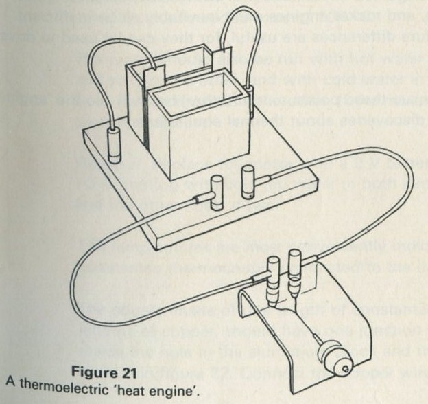
Figure 21: A thermoelectric heat engine.
Full Size Image
More of something good may be better
But if cold water is put in the other can, the motor runs well, and, if ice is used, it runs even better. Indeed it will run if the hot can is filled with cool water from the tap as long as the other can is filled with solid carbon dioxide (dry ice). It will not run if each side of the device is equally hot or cool.
Q1 If the motor is running now, will it still be running in an hour's time? Why not?
Q2 Where does the energy to run the motor come from?
Q3 Why is there a heat flow from the hot can into the semiconductor sandwich?
Q4 Why is the sandwich cooler than the hot can?
Q5 Would the motor go on running if the cold can were not there?
Q6 Why must some heat flow into the cold can? Is this energy available to run the motor?
Q7 Is all the energy going out of the hot can into the semiconductor available to run the motor?
This engine cannot help but be inefficient to some extent. We shall return to the inefficiency of such engines later on, in Part Six, and outline why steam engines, petrol engines, gas turbines, and rocket engines must inevitably all be inefficient. We note now that temperature differences are useful, for they can be used to drive engines.
In this Part, we shall not pursue these points much further, but will use the engine to illustrate Joseph Black's discoveries about thermal equilibrium.
Demonstration: 9.6 A heat engine
1072 semiconductor thermopile unit
1023 solar motor
1004/1 voltmeter (1 V)
542 thermometers ( -10 to 110�C) 2
507 stop watch or stop clock
176 12 volt battery (to give 2V d.c.)
1001 galvanometer (internal light beam)
1054/2B copper wire, 32 s.w.g., and constantan wire 32 s.w.g.
77 aluminium block
1053 slab of expanded polystyrene, Sellotape, card
supply of ice and of boiling water, salt, or solid C02
1000 leads
The flat surfaces of the cans which will be in contact with the semiconductor thermopile should be lightly greased to obtain good thermal contact, and then held against the thermopile with a rubber band. The spindle of the motor should be passed through the centre of a small strip of card ( 40 mm � 10 mm), to act as a rotation indicator, and the motor connected directly to the thermopile unit.
Fill one can with boiling water. After a minute or two, try to start the motor by turning the spindle. When it is running, fill the other can with boiling water. The motor should stop within half a minute. Note that the thermopile unit will be permanently damaged if the temperature of the junctions is allowed to exceed 100�C.
The motor should also be run with hot water in one can and ice (or ice and salt) in the other, and with cold water in one can and ice and salt or solid carbon dioxide in the other. If the motor fails to run, a meter can be used instead.
Reversal. Replace the motor with a 2 V battery which will deliver up to 10 A, starting with cold tap water in both cans. One can warms up and the other cools down.
The temperatures are most conveniently indicated using a copper-constantan thermocouple connected to the light beam galvanometer.
The couple, made of one length of constantan wire joined to two lengths of copper, should have one junction at a steady temperature inside the hole in the aluminium block and the other in one of the two cans as in figure 22. Connect the copper wires to the galvanometer.
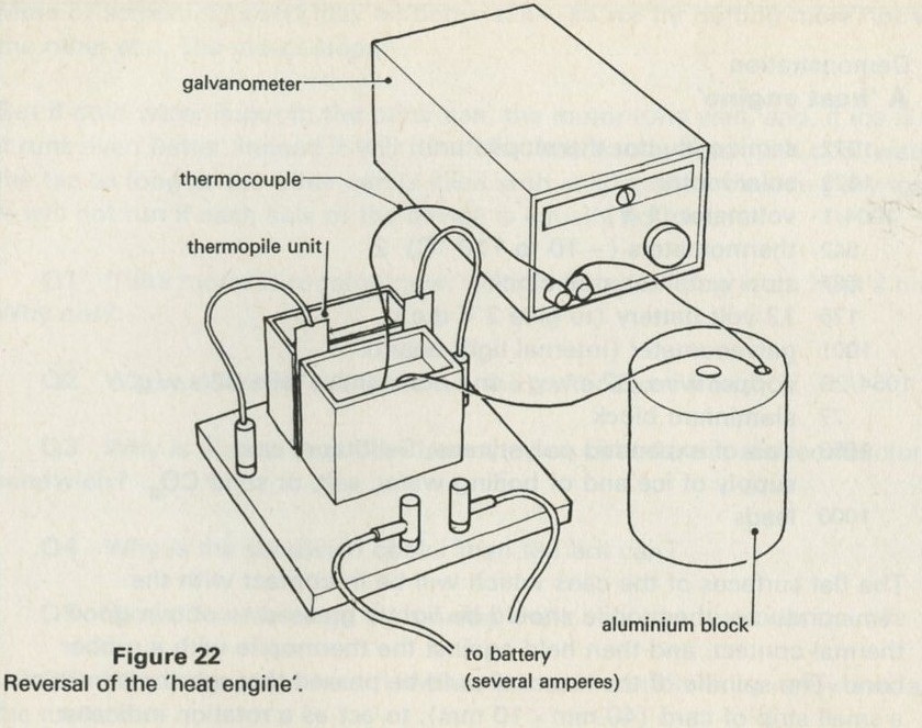
Figure 22: Reversal of the heat engine.
Full Size Image
(If a single junction couple is used, the galvanometer reading will drift as its terminals are warmed by the lamp in the galvanometer.) Use the x .01 position of the galvanometer initially, setting the zero to the centre of the scale. Alter the sensitivity if necessary to keep the deflections on the scale.
Follow the rise and fall of temperature of the water in the two cans by moving the couple from one to the other. See figure 23.
Thermal equilibrium
Disconnect the battery, and follow the return to thermal equilibrium. It is quicker to remove the cans from the sandwich and hold them directly in contact, using a rubber band. Stand them on an insulating surface, such as a piece of expanded polystyrene.
Since this experiment will bring out the very possibility of measuring temperature, it is best to describe what is happening without using the term. Instead, one can say that the galvanometer indication is big or small, this way, or the other way.
If the slow approach to equilibrium tries students' patience, mix the two lots of water!
Thermal equilibrium
Q8 Now imagine a film of the thermocouple device running a motor, but shown backwards. What would it seem to show? Say what energy transfers would seem to be taking place.
Interestingly, the reverse of the heat engine experiment can happen. The motor, run backwards as a dynamo, does not actually deliver enough current to produce an observable effect, so we replace it by a battery. When this is done, with equally cool water in each can, one lot of water grows warmer, and the other lot grows cooler.
This result may seem surprising, for we are all very accustomed to the inexorable one-way cooling down of hot things and warming up of cold things.
But if the battery is taken away, there are no surprises. Heat flows once again from the hot can to the cold can. A thermocouple connected to a meter, and placed alternately in each can, gives meter indications that are, at first, large but in opposite directions for the two cans. As time goes by, the two indications both become more and more nearly the same. See figure 23. Incidentally, the device is itself a thermocouple, but one between two sorts of semiconductor.
Note that so far as the conservation of energy is concerned (the basis of the First Law of Thermodynamics), energy could flow from cold to hot, as long as the same amount of energy left the cold object as reached the hot one.
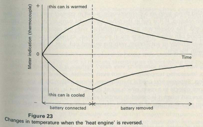
Figure 23: Changes in temperature when the heat engine is reversed.
Full Size Image
But, without external assistance, it never does. The approach to thermal equilibrium is one-way only. This is the theme of the Second Law of Thermodynamics, which will concern us more and more in this Unit.
Just now, we use the device to illustrate a third point, called the zeroth law of thermodynamics.
The First Law and energy conservation. See Appendix A for a discussion of the difference between the conservation of energy and the First Law.
The zeroth law. Since the First Law stole the number one, this yet more basic law was given the number zero. It says that if A is in thermal equilibrium with B, and B with C, then A will be in thermal equilibrium with C.
The zeroth law
What is thermal equilibrium? Objects in contact, like the warm and the cold cans, usually change their behaviour for a while. But soon all such changes stop, and the two are in equilibrium.
Suppose a third thing, such as a thermocouple, is put in contact with one can, and gives a certain reading. If it is put in the other, before the cans are in equilibrium, its reading changes. The couple was not in equilibrium with the second can. If it is put in the second can when the cans are in equilibrium, its reading doesn't change. The couple was already in equilibrium with the second can, just by being in equilibrium with the first.
Is this a long way of saying something very easy? Perhaps it is. But unless these things are so, measuring temperature is not even possible, indeed temperature means nothing. Suppose you used a thermometer whose indication is, say, 20�C, to find all those objects in a room which are at 20�C. That is, the thermometer indication stays put when it is placed in contact with them. Then the law we are thinking about says that none of them will change if they are put in contact with one another.
A set of objects of which we wish to say, all these are at the same temperature, must have something in common. And that something is that if they are put in contact, they will all be found already to be in thermal equilibrium.
This is called the 0th, or zeroth, law of thermodynamics. It is simple, but basic. If it were not so, a thermometer could give different readings for two things which were in equilibrium. Or perhaps one would find that of two things with the same reading, one of them was the hotter, because heat flowed from it to the other. Either event would make temperature measurement as we know it a useless procedure, because it would tell us nothing about the future behaviour of the bodies involved.
An analogy: getting on with someone
If A gets on well with B, and B gets on well with C, does A get on well with C? We could not be sure, so it would be impractical to think of measuring people so as to put each onto a scale of getting on well with others, and using the scale to predict who would get on with whom.
Q9 What does it mean, to say that two things are at the same temperature?
Q10 If two things are at the same temperature, do they contain equal amounts of energy?
Scales of temperature
Temperature exists is the message of the zeroth law. Making a scale of temperature, that is, putting a number to it, is a different matter.
Many scales have been invented, and many substances have been used in thermometers. Each scale, be it Celsius, Fahrenheit, Reaumur, or Kelvin, depends on deciding what number to assign to the temperatures of some things, such as ice, boiling water, or the lowest temperature possible, absolute zero. Each substance marks off by its changes, whether of volume, pressure, resistance, or some other property, the temperature between these fixed points. Any one thermometer can now be used to tell whether one object is hotter than another, according to how the physical property used to indicate temperature differs when the thermometer is put in contact with each in turn.
There remains, though, the question of assigning values of the temperature to the values of the physical property being used. If mercury in a thermometer placed in warm water can be seen to have completed half its expansion from ice temperature (0�C) to steam temperature (100�C}, it may seem sensible to assign the temperature 50�C on the mercury scale to that amount of expansion. But doing so is a matter of arbitrary decision, convenient but not absolutely necessary.
Furthermore. there is no guarantee that a coil of resistance wire, placed in the same warm water, will be found to have completed just half its increase of resistance from 0�C to 100�C. If the increase is less than half complete, the resistance coil temperature of the water will be (by the same decision) less than 50�C, disagreeing with the mercury expansion temperature.
These disagreements are usually not large, and their details are mainly important only in accurate work, or to thermometer designers. The existence of such disagreements indicates that we do not have here a fundamental basis for setting up a temperature scale. So we say no more about such temperature scales, though much of the rest of the Unit (especially Parts Four and Five) will pursue the problem of finding a fundamental basis for the idea of temperature measurement. This inquiry will lead us to the absolute, or Kelvin scale of temperature.
The large scale and the small scale
In the rest of this Part, we shall ask and begin to answer such questions as What is going on when things reach thermal equilibrium?, How do atoms come to share out energy so that the temperature is uniform?, and What is the difference between hot and cold so far as atoms in a body are concerned?
We shall be thinking about the large-scale (macroscopic) events discussed above and trying to form a small-scale (atomic, microscopic) picture of what is going on.
Einstein's model solid
To think about the questions raised above, we need to fix attention on something definite. It is no use trying to think about gases, solids, and liquids all at once, for each has its own rules for the motion and energy of its atoms. We need to find one definite picture of how atoms share energy in one kind of material. And it had better be as simple a picture as possible, to start with.
The best theoretical physicists often succeed because they can invent a really simple model which nevertheless gives useful ideas about complicated reality. It was Einstein who proposed the simple model we shall talk about. It is a model of a solid.
Q11 In a solid crystal such as sodium chloride, the ions are held in place by balanced forces acting on each ion. If one ion is displaced and released, how will it move?
Q12 Would you expect the oscillations of one ion to affect others nearby?
Q13 If all the ions in a row were oscillating in unison except one, what would you expect to happen to that one?
Einstein suggested thinking of atoms or ions as being fixed in place in a solid and vibrating as harmonic oscillators (remember Unit 4). In general they do not but it is much simpler to discuss their energy if we imagine a model in which they do. This is because such an oscillating atom can only have one of a series of definite energies, and these energy levels are equally spaced, like the rungs of a ladder. In Unit 2 you saw that there was experimental evidence that the electrons within atoms could be in only one out of a series of energy levels at a time. Those levels were not equally spaced. We are now talking about the energy of the atom when the whole atom is oscillating back and forth inside a crystal, not about the energy of electrons within the atom. These oscillation levels are equally spaced, if the oscillator is harmonic. The next experiment offers some experimental evidence to support this assertion. A theoretical reason to support the assertion can be found in Unit 10, Waves, particles, and atoms.
Einstein then introduced a further simplification that was very helpful, even though it was obviously wrong. It takes real cleverness to dare to do that, and to choose the right way to make the model wrong. The trick is to leave out those complications which won't affect the answers to the questions one is interested in (without knowing what those answers are!). Einstein's model achieves this for the answers we shall obtain.
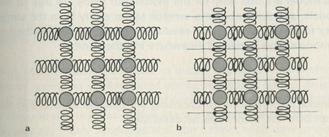
Figure 24: Models of a solid
Full Size Image
a A balls and springs model of a solid (later developed theoretically by Born and von Karman, in an improvement upon Einstein's arguments).
b Einstein's model, with nearly rigid prison cells around each oscillating atom.
Figure 24 illustrates this simplification. As the answer to question 13 suggests, the oscillations of one atom in a regular array, all linked by springy bonds as in figure 24 a, will affect the oscillations of others. In fact, figure 24 a is like a wave model of trolleys joined by springs (as used in Unit 4) but extended to two or to three dimensions. Indeed, those who developed Einstein's simpler arguments had to argue in terms of wave energy travelling all through the crystal. The trouble is that the energy levels of such linked oscillators affect each other so much that one cannot speak of the energy on one atom at all. Einstein's idea was to imagine the atom-oscillators not as if they were linked together but as if each were enclosed in a rigid prison cell, as in figure 24 b. But this was going too far, for then energy Would not be transferred from one atom to another at all, and there certainly would not be any heat flow to be discussed. So Einstein made the model a bit fuzzy at the edges, and allowed himself to imagine the walls of the prison cells as being just a little flexible, but not so much that the motion of one atom governed that of another nearby. Then energy could go from atom to atom, but the energy levels of each would be unaffected by the motions of any of the rest of the atoms.
Please don't think that Einstein proposed the model as a good way of imagining the arrangement of atoms in a solid. He proposed it as the simplest model he could think of which would still allow him to argue about heat flow and thermal equilibrium. As our present interest is in these matters, and not in the nature of solids, it is sensible to adopt the simplest possible model. But remember, although we shall talk of the energy of one atom, the model was invented to make that possible. For a real solid, it is usually not possible to think like that at all, and one must imagine compression waves travelling through all the solid and think of all the atoms sharing the energy cooperatively. (Real solids are like communist societies - all for one and one for all - while Einstein's model is like that simplified economic theory which supposes that there are many independent small manufacturers and shopkeepers, each acting independently of the rest, except for some flow of money between them. Their wealth can be counted up for each individual. In the ideal communist society the wealth belongs to everybody.) Some of the results of thinking about the model are true only for the model, but many are true of much more complex models, and just happen to emerge rather easily from the simple model. We shall try to make it clear which results are of each kind. Analogous arguments using models have appeared elsewhere in other Units.
See Appendix B for reasons for choosing the Einstein model, and for more about how the theory can be developed.
Demonstration 9.7 A ladder of equal energy levels
We said that an atom vibrating like a harmonic oscillator has an energy limited to one of a series of equally spaced values. The energy level spacing is actually hf, where h is Planck's constant and f is the frequency the oscillator has in the ordinary theory of oscillators (2πf= √(k/m)) where k is the spring constant and m the mass).
Imagine the levels to be like the rungs of a ladder, as in figure 25. There is a lowest rung, rung zero, and others above it. If the atom passes from rung one to rung two it has to acquire one lump of energy, magnitude ε. But on another occasion it may pass from rung five to rung four: it then gives up the same amount of energy ε.
An oscillating atom may absorb the energy needed to jump from one level to another, from some light. hf (again) gives the energy absorbed, the frequency f being that of the light. A spectrum of light, that has passed through some oscillating atoms that have absorbed energy from it shows dark lines at particular frequencies f, and these frequencies yield evidence of the energies hf absorbed from the light. (In Unit 4 we argued about this for the absorption of infra-red radiation by sodium chloride.)
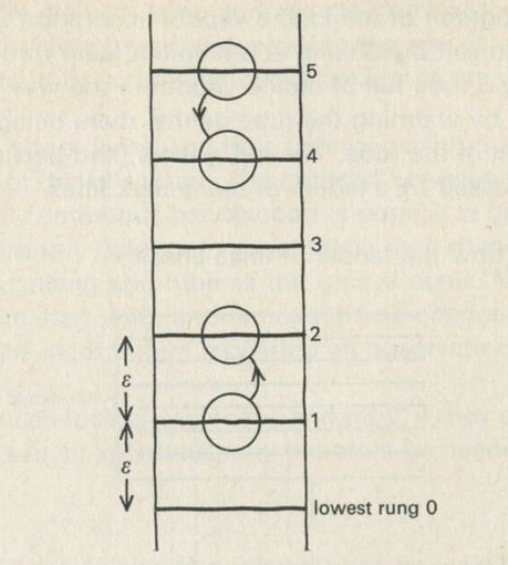
Figure 25: A ladder of levels
Full Size Image
A solid, even a transparent solid, is quite unsuitable for showing the equally spaced ladder of levels. As we explained above, real solids are not much like the Einstein model made of many independent oscillators. For a demonstration of the ladder, the best thing to use is a gas of two-atom molecules, like iodine, I2. Being in a gas, the molecules are nicely separated and don't affect each other's vibrations. Being made of two atoms, each molecule can vibrate in and out like two masses joined by a spring.
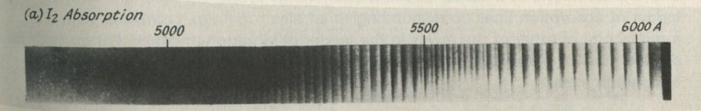
Figure 26: Part of the absorption spectrum of iodine vapour.
Full Size Image
From Gaydon, A. G. (1968) Dissociation energies and spectra of diatomic molecules, Chapman & Hall.
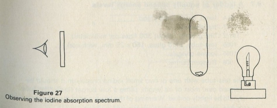
Figure 27: Observing the iodine absorption spectrum.
Full Size Image
Figure 26 is a photograph of the iodine vapour absorption spectrum. You can see the spectrum for yourself by looking at a filament lamp through a diffraction grating, and putting a tube full of iodine vapour in the way as in figure 27. The vapour is produced by warming the tube gently, there being one small iodine crystal in the bottom of the tube. The red, yellow, and part of the green regions of the spectrum are crossed by a ladder of many dark lines.
Figure 28 suggests how the ladder of lines arises.
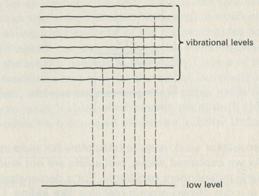
Figure 28
In the warm iodine vapour, nearly all molecules are in the lowest state of electron energy, and many have the least possible vibration energy. A molecule can absorb energy by jumping to a higher state of electron energy, but the excited molecule can also vibrate in one of a ladder of vibrational energy levels. So there is a whole ladder of absorption lines corresponding to an electron jump, combined with a jump to one or other of the levels in the ladder of vibration energies that go with an excited state of the electrons in the 12 molecule. Ladders of levels give ladders of absorption lines.
Demonstration 9.7 A ladder of equally spaced energy levels
94A lamp, holder, and stand
27 transformer
191/2 fine grating (about 300 lines per millimetre)
1055 test-tube, hard glass, 150 � 25 mm, with cork
1056 iodine crystals
508 Bunsen burner
The test-tube with one or two small iodine crystals in it should be warmed over most of its length, using a low burner flame. The tube should be lightly corked. Warming of the lower part of the tube should be continued until the iodine vaporizes. The tube may now be supported in front of the line filament lamp and the spectrum of the emerging light examined by holding the grating close to the eye. It is necessary to warm the sides of the tube to prevent condensation of the iodine vapour there.
If the vapour is too dense, too little light comes through for much to be seen. If it is not dense enough, the contrast between the absorption bands and the continuous background is poor. It is best to warm the tube until a strongly coloured vapour fills it, and then to watch the lamp through grating and tube as the vapour cools. Make sure the tube is clean to start with, and remove iodine condensed on the sides by warming the sides before repeating an observation.
Four students can look at each lamp and tube, if they each have a grating. Four or more sets of apparatus may therefore be needed, with sixteen gratings.
Over-simplifications in the vibrational energy level story
There is not one single level from which the 12 molecules jump to higher levels, but the ground state is split into vibrational levels too. At moderate temperatures, the population of vibrational levels above the lowest is not very big, but careful inspection of the spectrum reveals at least two ladders of lines corresponding to jumps from the two lowest vibrational levels. See figure 29 a.
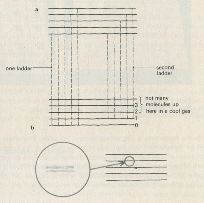
Figure 29
Full Size Image
In addition, the 12 molecules can also rotate. This splits each vibrational level into many finely spaced rotational levels (figure 29 b). As a result, each absorption line is really many closely spaced lines. Through a grating the lines appear broader than, for example, the absorption lines in sodium vapour, but the rotational lines are not resolved.
Zero-point energy
As stated above, the energy level spacing of a quantum harmonic oscillator with a classical frequency f is hf. The lowest level, however, has energy not equal to zero but to �hf. The other levels have energy (1 +�)hf, (2+�)hf, and so on. Actually, the ladder in figure 25 has been drawn with its lowest rung half a rung spacing above the ground.
A game of chess with quanta for chessmen
The chess board (though it has only 36 squares) in figure 30 represents the array of atoms in a solid, each square, like each atom, having a fixed site within the whole.
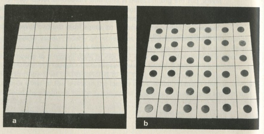
Figure 30: A chess board of atomic sites in a solid. Photographs Michael Plomer
Full Size Image
Each square represents a site where there is an atom. The energy of an atom at one site will be represented by piling counters on that site. No counters on a site means that the atom at that site is in its lowest energy level. One counter is added to represent lifting it to the first level, another to represent lifting it to the next, and so on. Figure 30 a shows the 36-atom solid with each atom in its lowest level.
Figure 30 b shows it with each atom in the next level up, with one counter on each site.
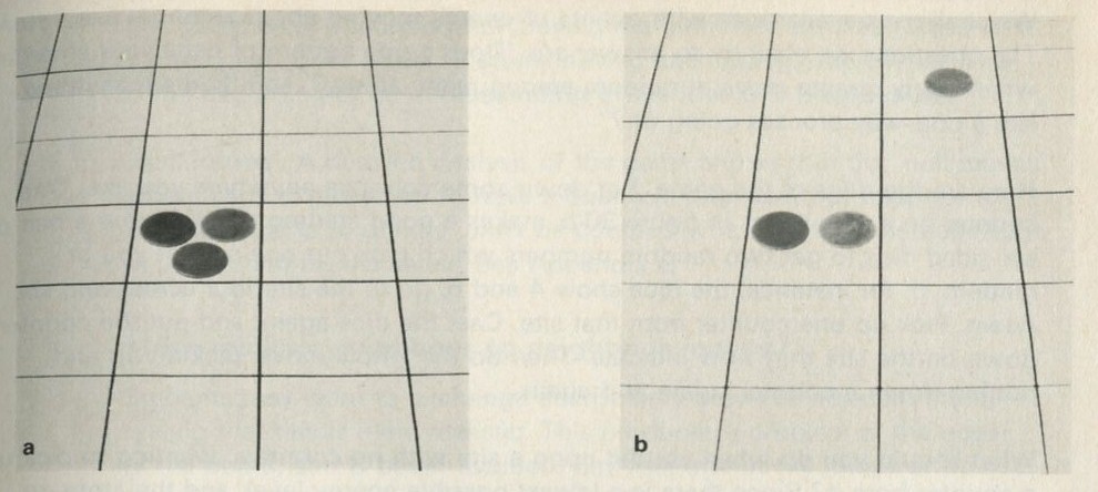
Figure 31: Transferring one quantum of energy. Photographs, Michael Plamer.
Full Size Image
How shall we represent energy passing from atom to atom? The energy levels are equally spaced. Therefore, if a counter is picked up from an atom in the third level (with three counters, so that it then has two and has dropped one level), the same counter can be put down anywhere else and will represent the atom it now joins jumping up one level. Figures 31 a and b show one atom going from level 3 to level 2, and another going from the lowest level to the first level above that, all by moving one counter.
If a counter, representing one quantum of energy, were not put down once it had been picked up, the total energy would have decreased. It must go somewhere; to begin with we shall investigate what happens when the solid is well insulated so that no energy leaks in or out. So a counter picked up from one site must be put down on some site or other.
The fact that the counters representing quanta (which are real bits of plastic or metal) are distinct from one another, is not true of quanta. But the moves could just as well be made by keeping a paper and pencil tally of the state of each atom, remembering to move one atom down an energy level for every other atom one moved up one level. The plastic counters just save one having to remember or write down the state of each atom.
Game: 9.8 Moving quanta at random
How shall we choose which atoms gain energy and which lose energy? The clue to Understanding diffusion in Part Three was that there were no rules other than those of chance: if atoms move about quite by chance, then diffusion will inexorably happen if there are many atoms involved. A predictable, one-way diffusion process emerges from total atomic chaos.
We shall try a similar idea with quanta of energy moving about amongst fixed atoms. The questions we shall try to answer are, Does a tidy pattern of behaviour emerge when many quanta move at random among many atoms? and Is there anything like a one-way process going on?
Here are the rules of the game. Put down some counters anywhere you like. One counter on each site, as in figure 30 b, makes a good starting point. Throw a pair of six-sided dice to get two random numbers which pick out one site for you at random. If, for instance, the dice show 4 and 6, go to the site four across and six down. Pick up one counter from that site. Cast the dice again, and put the counter down on the site they now indicate. Then do the whole move, picking up and putting down a counter, again and again.
What should you do when you hit upon a site with no counters, wanting to pick up a counter from it? Since there is a lowest possible energy level, and the atom on that site is already in this level, it can go no further down. You will have to try again for another site, perhaps several times, until you find one with a counter to pick up.
The game does have definite rules. They are meant to achieve chaos. There are no rules saying where a quantum (counter) must go from each particular place: it may go anywhere. In that sense, there are no rules, or if you prefer, only that of chance.
Game: 9.8 Moving quanta at random
    1053 counter (tiddlywinks are suitable) 36
    1055 dice 2
    1054 graph paper 2 sheets
Have a six-by-six grid ruled on one sheet of graph paper for each player, the squares being at least 30 mm on a side. It will be convenient to have the results of at least eight games available for averaging, so up to three hundred counters are needed.
The other sheet of graph paper is needed for recording a bar chart of the number of sites having no counters, one counter, two, and so on. It is convenient to plot such charts after twenty, sixty, and a hundred moves.
The rules of the game are given above, in the text. The game, and others like it, will shortly be shown on film, played by a computer using 900 sites. The purpose of playing the game with a 36-site board is that students should be clear about what the computer is doing, and see for themselves at first hand some of the expected and the unexpected results. If they use small numbers themselves, they will more easily appreciate the need for the large numbers used by the computer.
It is particularly important that playing the game should teach them what the bar chart of numbers of atoms having each energy represents. This is the beginning of an understanding of the idea of a distribution.
Null moves. A detailed analysis of the game shows that the null moves, when a site is picked on to have a quantum removed, but happens to have no quanta to donate, must be counted when the average behaviour of the system is calculated. See Appendix C.
More realistic neighbour to neighbour moves?
Students may want to exchange energy only between adjacent atoms, feeling that this is more realistic. This produces a problem at the edges of the board, and is better avoided. Say that one of the jumps of a quantum in the game might be the result of several steps in a real crystal, and that our aim is to use as simple a rule as possible. The diffusion game was not realistic either, but it predicted the average behaviour quite well even so.
Other random number generators
Dice serve well for a six-by-six board. A box containing balls numbered from one up to the total number of sites is also good, if the balls are jumbled between moves and are returned to the box after each draw. Numbered cards in a box are simpler, but experience suggests that they are not usually easy to shuffle well. Tables of random numbers are best avoided, for students are still learning what random means. It must be clear to them that nobody could have predicted beforehand how their own game would go.
How many squares?
The smaller the number of squares the quicker the game but the less reliable the results. 36 is the minimum. 64 is quite nice, but 100 is too many, for the game has then to go on for several hundred moves before it reaches statistical equilibrium. As the games will, in any case, be shown on a computer-made film with 900 sites it is probably best to keep to 36 sites now.
Atoms and oscillators
As indicated at the end of this Part, each atom can oscillate independently in each of three perpendicular directions. Thus, one site, corresponding to one oscillator, represents only one-third of an atom. Strict usage would require oscillator to be substituted for atom in all of this Part.
What happens in the game?
When you play the game you may notice a number of things. As you ought to have expected, the nice tidy one-counter-per-site pattern soon vanishes. And it never returns: the game leads, one-way only, away from such tidy patterns.
After about a hundred moves it is interesting to ask whether another hundred moves will make any more change. In one sense, obviously the answer would be yes. If you go on and on, some, at least, of the atoms which now have, say, two counters will have some other number of counters. The counters keep on moving. Yet, in another sense, not much more change happens, however long you go on after the first long run of moves.
Q14 Suppose you made the following records after 100 and 200 moves:
A the locations of sites with, say, two counters.
B the number of sites with, say, two counters.
Which record would be about the same each time, do you think?
The distribution of quanta among atoms
To start with, you may have had 36 sites each with one counter. No sites had no counters, and no sites had two, or any larger number of counters.
After a while, some sites have no counters, fewer than 36 have one, some have two, and so on. A good way to follow such changes is to plot bar charts with columns whose heights represent the numbers of atoms having no quanta, one quantum, two quanta, and so on. This is called the distribution of the atoms among the possible energy levels.
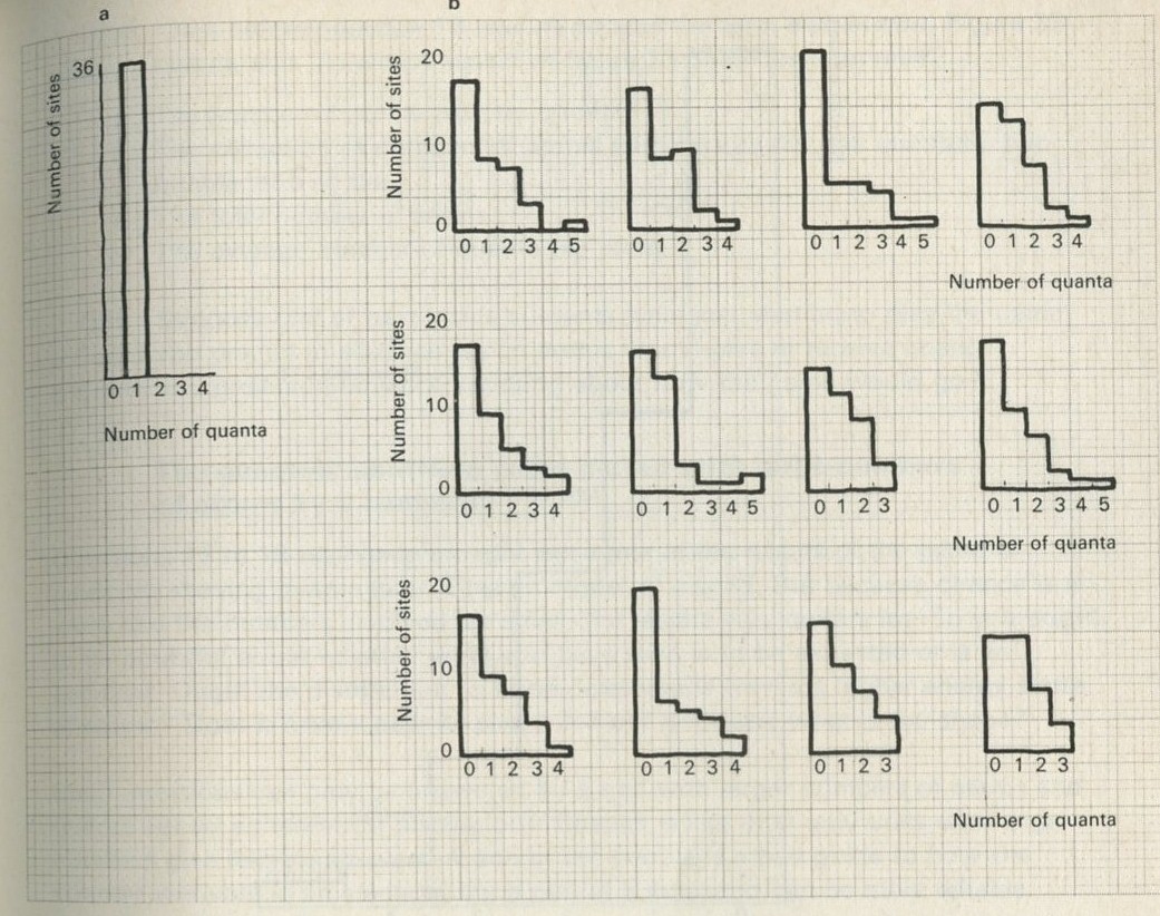
Figure 32: Twelve sample games (36 sites, 36 quanta, 100 moves) played by computer. a Initial distribution. b Distributions after 100 moves.
Full Size Image
Figure 32 a shows what the bar chart looks like if you start with one counter on each atom - a single column 36 units high. Figure 32 b shows what happened to the distribution after 100 moves in each of twelve different trials of the game. Figure 33 shows the average of these twelve games.
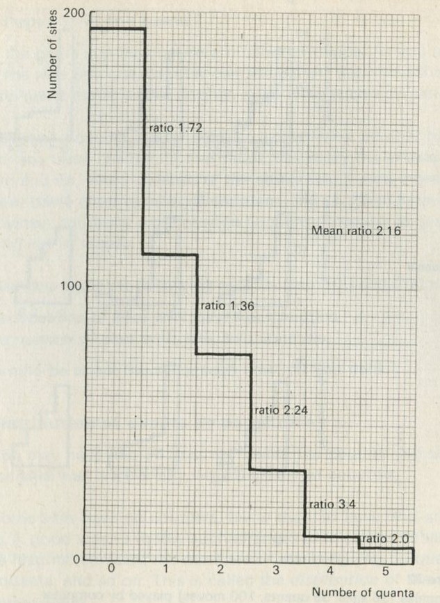
Figure 33: Total of 12 computer samples (36 sites, 36 quanta, 100 moves in each sample).
Full Size Image
Q15 Look at figure 33, or at the average of the bar charts obtained in your class. Suggest a rule about whether the numbers of atoms with n quanta will be more than, fewer than, or the same as with n + 1 quanta.
Q16 Is the difference between the number of atoms having four quanta and the number having three quanta the same as the difference between the number of atoms having one quantum and the number having none?
Q17 Speculate: what might be true of the ratios between the numbers of atoms in adjacent columns of the chart, but for chance variations because of the small total numbers involved?
Q18 Just before question 15, we introduced the term distribution. Figure 33 shows a distribution. To which aspect of figure 33 does this term refer?
- a The number of atoms with no quanta.
- b The collection of numbers of atoms with no quanta, one quantum, two quanta, and so on.
- c The total number of atoms.
- d The average number of quanta per atom.
Q19 Suppose one of next year's students were just starting to play the game.
- a Could you predict in advance which atoms would give or receive quanta?
- b Could you predict in advance anything about how the game would go?
The quantum shuffling game played with large numbers of atoms by a computer
Questions 15 to 19 may have brought out some of the results of the game of randomly moving quanta in an Einstein model of a solid. But because chance is at work and the numbers involved are small, the results vary quite a lot. So you ought to be doubtful about whether what you have seen is to be expected or is an accident. Ought the distribution to slope downwards towards higher energy states of atoms? Does it have a definite shape or not? If it does, what is the shape?
Such questions can only be answered by a trial with larger numbers of atoms and quanta (or by a theoretical discussion). Chance is like that: only trials with large numbers give reliable answers. A poll of ten people is a bad guide to how the country will vote in an election, but a poll of a thousand can be more reliable.
Sometimes it is possible to calculate in advance what to expect. This is possible for the number of times zero will turn up at roulette, but not for the number of votes in an election. It is possible to make such a calculation for the quantum shuffling game, but it is not easy. Part Five indicates how it may be done, and the calculation is given in Appendix B. For many problems, calculations are too difficult or impossible, and they are often tackled by making many random trials to see what happens. The problem of the most likely length occupied by a polymer molecule that can coil and uncoil at random, has been tackled in this way, for instance. This way of going about a problem is called, for obvious reasons, the Monte Carlo method. The advent of computers which can rapidly make many random trials according to certain rules has greatly increased the popularity of Monte Carlo methods.
We arranged for a computer to play the game you have just tried, but with 900 sites and 900 counters. The computer simultaneously made a film of what was happening in its head, so that you can see how the quanta move about and what happens to the bar chart showing the distribution.
computer films
The six short films on one reel are:
- 1 Equilibrium of randomly shuffled quanta
- 2 Different initial arrangement of quanta
- 3 Fewer atoms and fewer quanta
- 4 The biography of one atom
- 5 A colder solid
- 6 Heat goes from hot to cold
The series is entitled Change and chance: a model of thermal equilibrium in a solid.
The first film starts by showing the game played very slowly for two moves, so that students may see that the rules are exactly the same as those they have used. Then the 900 quanta are shuffled more and more rapidly for 10 000 moves, by which time the bar chart has changed to the expected exponential form. Then a further 10 000 moves follow, showing that statistical equilibrium has been reached, for the distribution (bar chart) merely fluctuates a little around a steady exponential shape. The average of the last 10 000 moves is then shown to be rather accurately exponential in form.
The second film shows that 900 quanta and 900 atoms reach the same final distribution even though they are differently arranged to begin with.
The third film shows that the final distribution has the same form if only 625 quanta and 625 atoms are used. The steepness of the distribution thus depends, in this model, on the number of quanta per atom.
The fourth film shows that the biography of one atom followed for 800 000 moves has much the same pattern as the distribution of numbers of atoms having various energies. Over a long period, one atom has zero quanta on as many occasions as it has one quantum, as, at an instant, there are atoms with no quanta rather than one quantum. This film is of importance mainly in Part Five. It can be passed over lightly now.
The fifth film shows the more steeply sloping distribution reached by 900 atoms sharing only 300 quanta.
The sixth film proves that 900 atoms sharing 900 quanta is hotter than 900 atoms sharing 300 quanta, for when these two are put together, energy flows spontaneously from the former to the latter, until they reach a common equilibrium.
Still pictures from the computer films of randomly shuffled quanta
In all, the computer made six short films, the series being called Change and chance: a model of thermal equilibrium in a solid. Figures 34 to 65 are still frames from the films, for you to inspect at leisure. (The frames are not prints from the film negative, but were made at the same time as the film, using the same data. The computer printed the pictures directly onto sensitized paper as well as onto film.)
Equilibrium of randomly shuffled quanta (figures 34 to 42)
In this film, the first, 900 atoms share 900 quanta, starting with one quantum on each atom. After making two moves in slow motion, to show that the rule used is the same as the rule we suggested that you should use in the game (9.8), moves are made at high speed until 10,000 moves have been made. The distribution has changed to a downward-sloping shape. Then a further 10,000 moves are made, during which the distribution fluctuates a little, but does not change its overall shape. Finally, the average distribution for the last 10,000 moves is calculated and displayed.
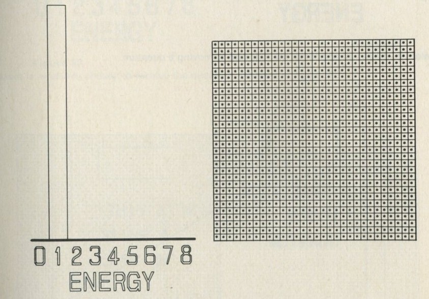
Figure 34: 900 atoms each with one quantum.
Full Size Image
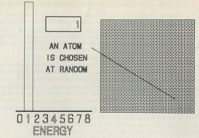
Figure 35: One atom is chosen as the first step in moving a quanta.
Full Size Image
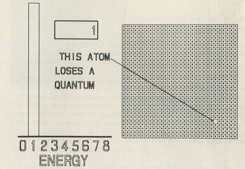
Figure 36: The atom chosen in Figure 35 loses a quanta.
Full Size Image
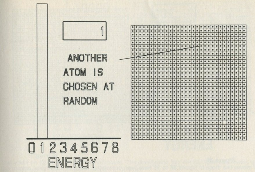
Figure 37: An atom is randomly chosen to receive the quantum removed in figure 36.
Full Size Image
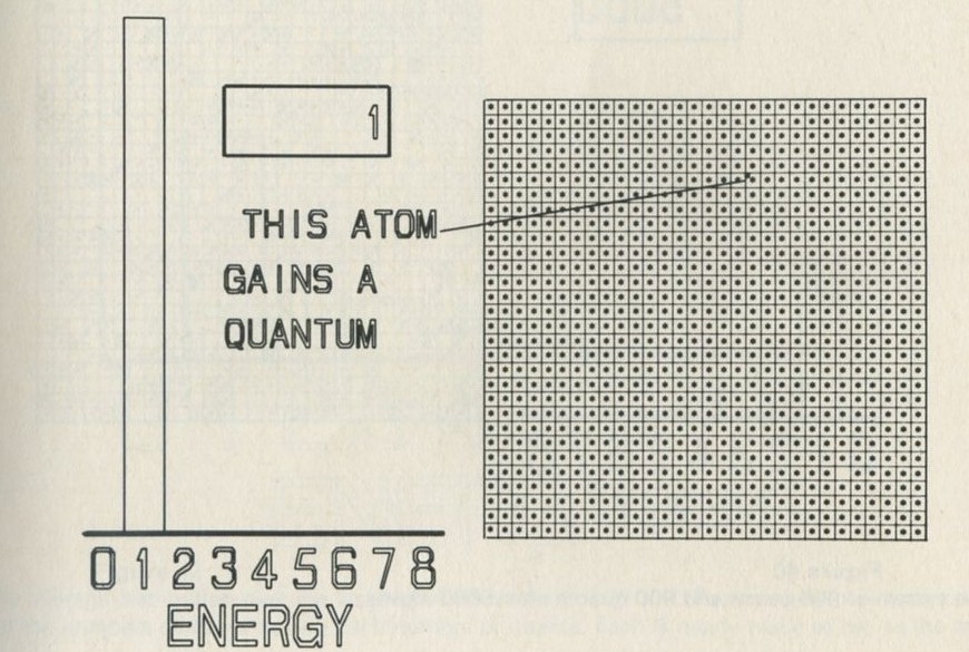
Figure 38: The quantum removed from an atom in figure 36 is given to another atom. One move is completed.
Full Size Image
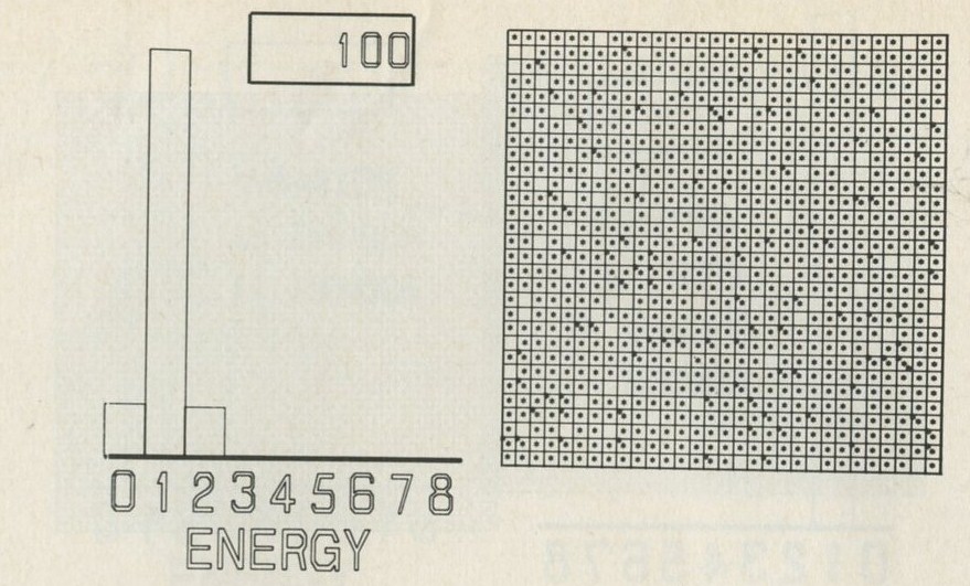
Figure 39: 100 moves like those in figures 36 to 38 have been completed. Much of the original pattern still persists but several atoms have no quanta or two quanta.
Full Size Image
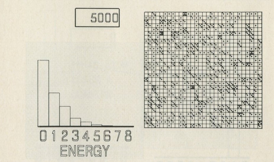
Figure 40: The system of 900 atoms and 900 quanta after 5000 moves.
Full Size Image
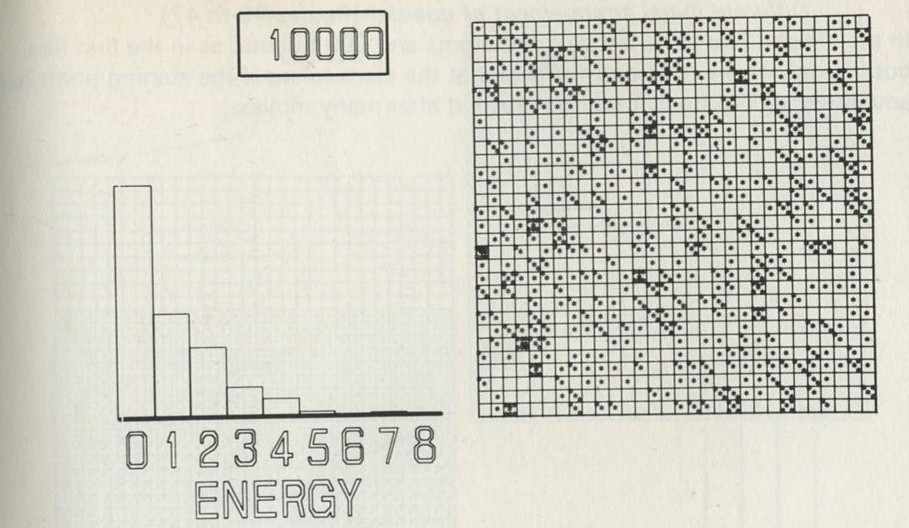
Figure 41: The effect on figure 40 of 5000 more moves. The distribution has not changed essentially, though individual atoms have different number of quanta.
Full Size Image
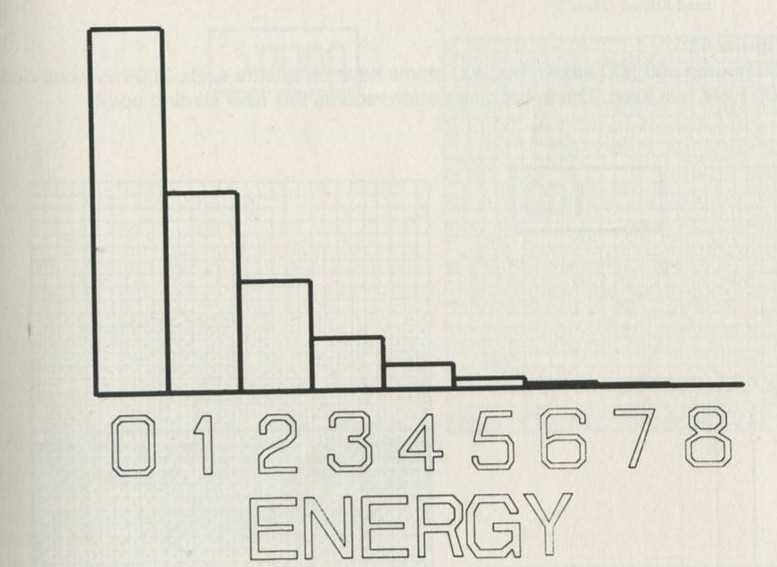
Figure 42: The average distribution over the last 10,000 moves out of 20,000. The numbers over each column are the numbers of atoms having each number of quanta. Each is nearly twice as big as the next.
Full Size Image
Different initial arrangement of quanta (figures 43 to 47)
In the second film there are still 900 atoms and 900 quanta, as in the first film, but the quanta are differently arranged at the start, to see if the starting point has any influence on the distribution reached after many moves.
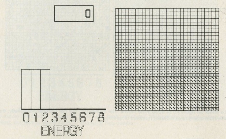
Figure 43: There are 900 quanta and 900 atoms, but 300 atoms have no quanta each, 300 have one quantum each, and 300 have two each. The initial distribution records this new starting point.
Full Size Image
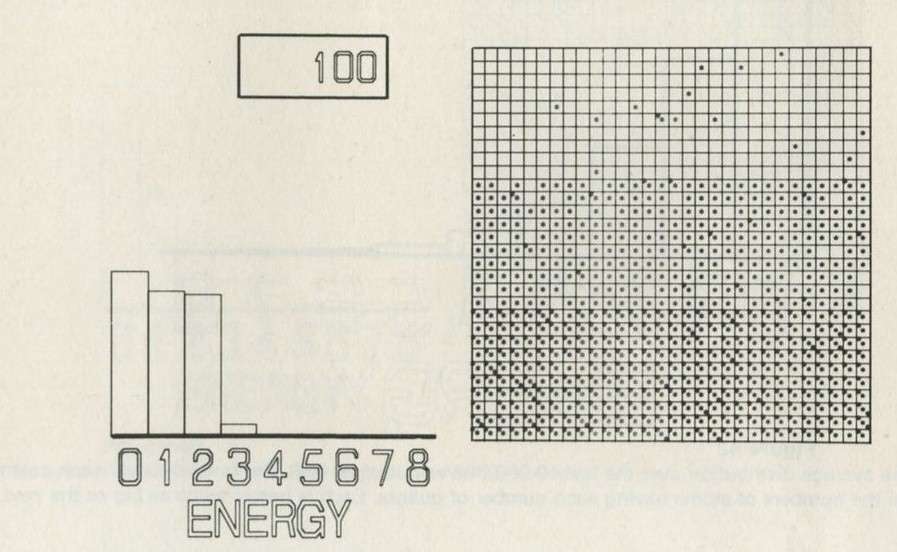
Figure 44: The system shown in figure 43 after 100 moves. The initial arrangement still largely persists, though some atoms have acquired three quanta each.
Full Size Image
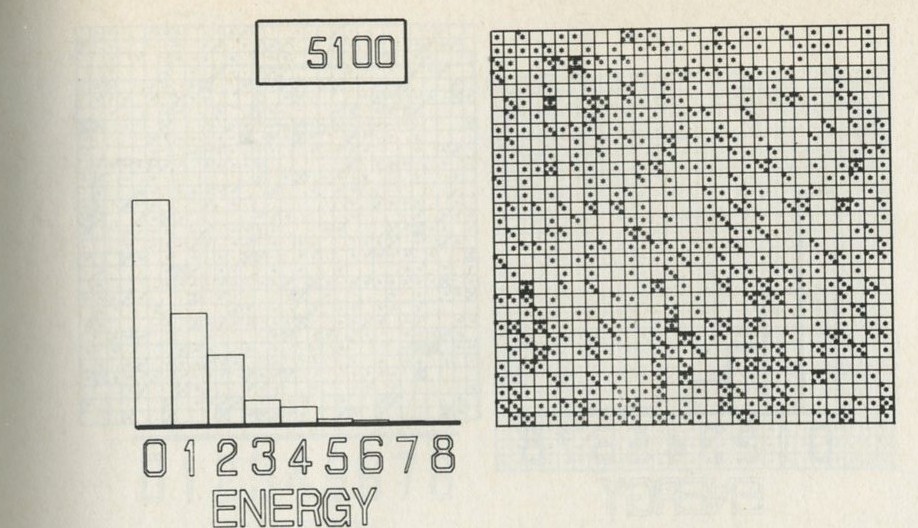
Figure 45: After 5100 moves the initial arrangement seen in figure 43 has quite vanished. The distribution is like that obtained in the first film, figure 40.
Full Size Image
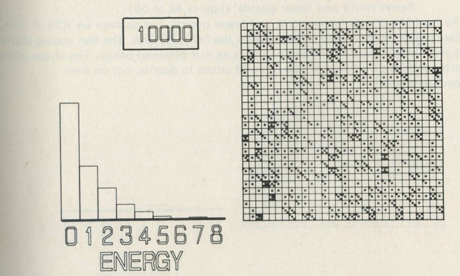
Figure 46: Approximately 5000 moves after figure 45 there is no essential change in the distribution, though individual atoms have different energies from those they had before.
Full Size Image
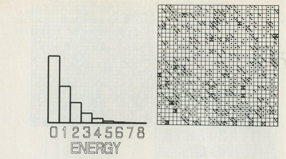
Figure 47: The bar chart shows the average distribution over the last 10 000 moves out of 20 000. This distribution is very much the same as that obtained in the first film.
Full Size Image
Fewer atoms and fewer quanta (figures 48 to 50)
The third film shows fewer atoms and fewer quanta, but as there are 625 of each, there is still one quantum per atom as in the first two films. The film shows that the final distribution is also the same in form as that obtained before. The shape of the distribution thus depends on the ratio of atoms to quanta, not on their absolute numbers.
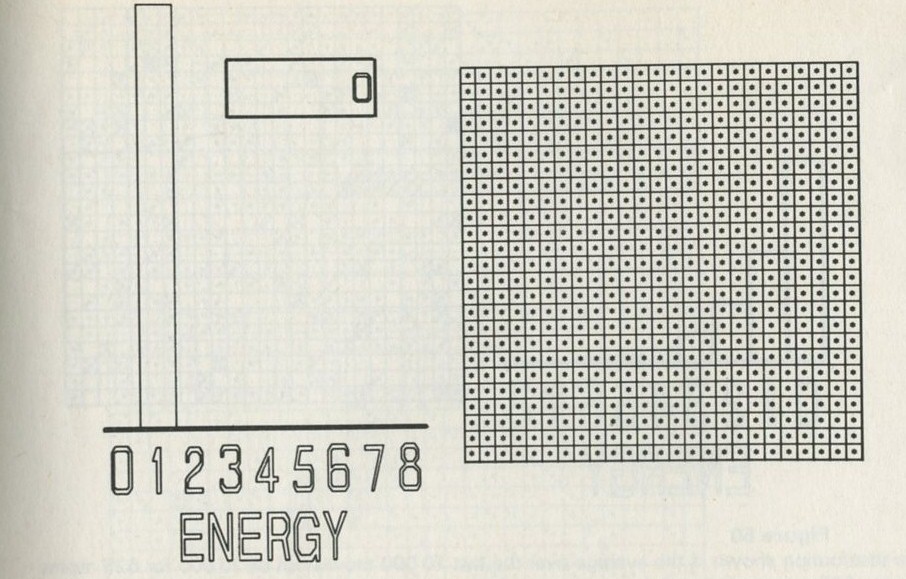
Figure 48: 625 atoms each have one quantum.
Full Size Image
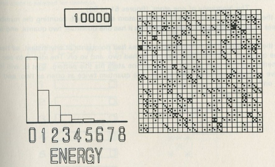
Figure 49: The distribution produced by random shuffling of quanta in the system shown in figure 48 is now changing no further.
Full Size Image
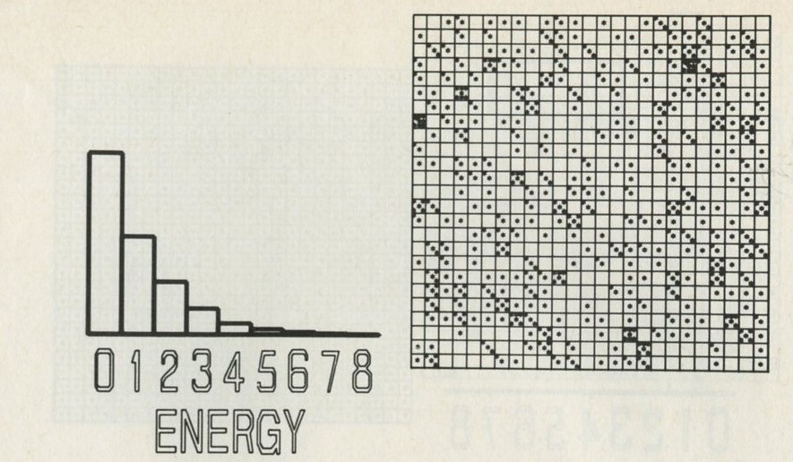
Figure 50: The distribution shown is the average over the last 10 000 moves out of 20 000 for 625 atoms sharing 625 quanta. It has the same form as those shown in figures 47 and 42. Each column is twice as tall as the one next to it.
Full Size Image
The biography of one atom (figures 51 to 56)
In the fourth film the fortunes of just one atom are followed, counting the number of times it has no quanta, the number of times it has one quantum, two quanta, and so on.
In the first three films, twice as many atoms had no quanta at any instant, as had one quantum, twice as many had one as had two, and so on. The idea is to see whether, as time goes by, the energy of one atom fits this pattern. That is, will it have no quanta twice as often as one, one quantum twice as often as two, and so on?
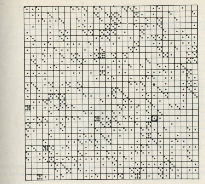
Figure 51: One atom is selected for attention.
Full Size Image
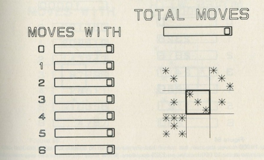
Figure 52: The selected atom has three quanta. No moves have yet been followed.
Full Size Image
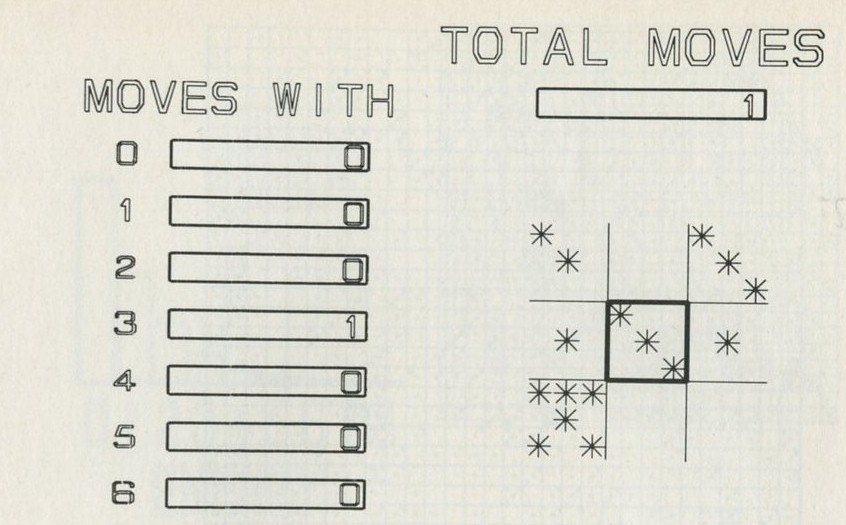
Figure 53: On the first move followed, the selected atom happens to retain its three quanta (the move affects other atoms). One count appears in the register for moves with three quanta on the selected atom.
Full Size Image
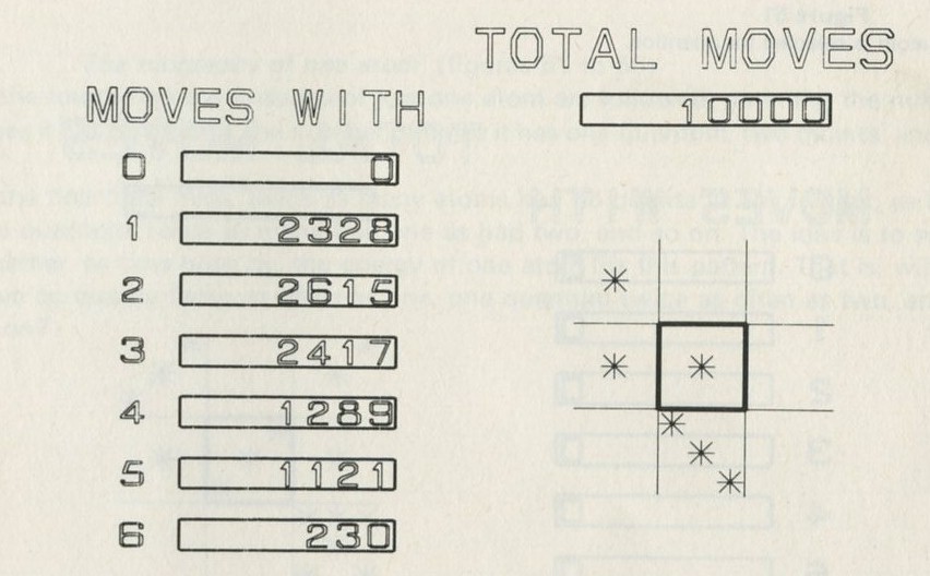
Figure 54: After 10000 moves, the atom has not yet had any moves with no quanta, though it has had one quantum as at the 10 000th move, on 2328 occasions. In the short run, chance can play many tricks. But as there are nearly 1000 other atoms, this one has probably only had about ten changes in its state so far.
Full Size Image
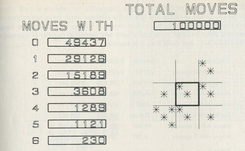
Figure 55: After 100 000 moves the registers show that the selected atom has had no quanta more often than one, one quantum more often than two, and so on. But the number in each register is only very roughly twice that in the next one down.
Full Size Image
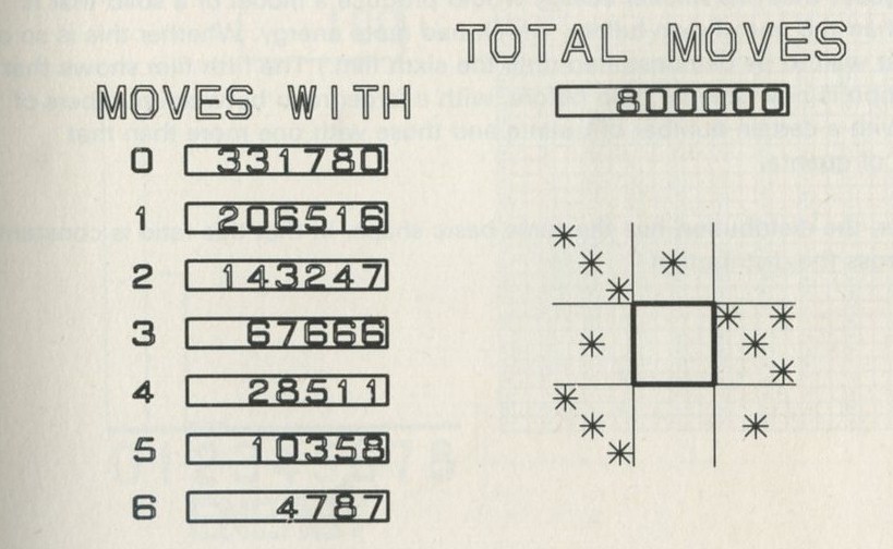
Figure 56: After 800,000 moves the ratios of numbers of moves with one, two, etc. quanta are rather nearer to two for more of the registers. But it would not be easy to be confident that this atom has no quanta twice as often as it has one, and so on for all numbers of quanta on the atom.
Full Size Image
The film had to stop after 800,000 moves (figure 56), for reasons of cost. But the computer continued to follow the fate of the selected atom up to ten million moves. Table 4 shows the results. By ten million moves it is fairly clear that in the long run one atom is twice as often to be found with any particular number of quanta, as it is to be found with one more than that number.
total moves            1 000 000   5 000 000   10 000 000
moves with 0 quanta      437 597   2 427 674    4 936 888
moves with 1 quantum     260 630   1 241 675    2 501 041
moves with 2 quanta      165 721     668 649    1 274 341
moves with 3 quanta       80 911     327 425      611 711
moves with 4 quanta       31 678     166 232      326 452
moves with 5 quanta       11 541      80 714      164 727
moves with 6 quanta        4 787      39 602       88 933
Table 4: Continuation of from four to ten million moves.
A colder solid (figures 57 to 60)
In the fifth film, only 300 quanta are shared among 900 atoms. (Perhaps you would guess that this smaller energy would produce a model of a solid that is colder than the one shown before, which had more energy. Whether this is so or not must wait to be demonstrated until the sixth film.) The fifth film shows that the distribution is now steeper than before, with a larger ratio between numbers of atoms with a certain number of quanta and those with one more than that number of quanta.
However, the distribution has the same basic shape, in that this ratio is constant right across the distribution.
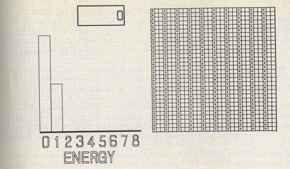
Figure 57: 900 atoms share only 300 quanta.
Full Size Image
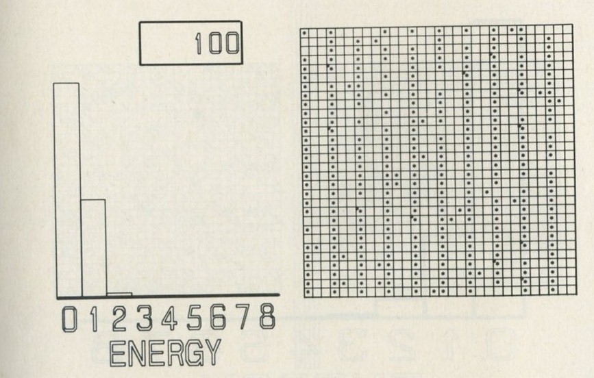
Figure 58: After 100 moves the original arrangement persists.
Full Size Image
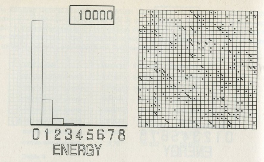
Figure 59: After 10 000 moves the distribution has reached a steady form.
Full Size Image
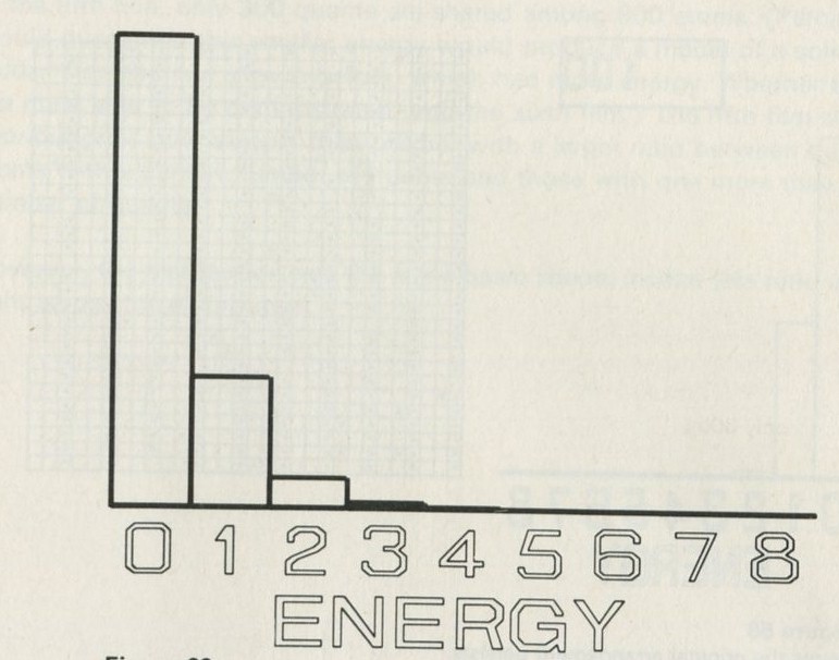
Figure 60: The average distribution, taken over the last 10 000 moves out of 20 000. It is steeper than that in figure 42, for 900 atoms and 900 quanta. That is, fewer atoms have large energies. There are tour times as many with no quanta as with one, and so on.
Full Size Image
Heat goes from hot to cold (figures 61 to 65)
In the sixth film, the model solid with 900 quanta and 900 atoms from the first film is allowed to exchange energy with the model from the fifth film, which has only 300 quanta among 900 atoms. One might expect the model with less energy to behave as if it were the colder of the two: this film shows that it does.
The two solids are first allowed to reach equilibrium within themselves, quanta being shuffled within each but not being allowed to pass from one to the other. It is as if there were an insulating wall of, say, expanded polystyrene between them.
Then the insulating wall is removed, and the computer is instructed to treat the two solids together as one large solid, shuffling quanta amongst all the sites in the combined system. Soon the quanta are evenly spread and the effect of this spreading on the two distributions of atoms among energy levels can be seen.
Quite by chance, energy goes from one to the other. The one which loses energy must previously have been the hotter of the two; the one which gains energy, the colder.
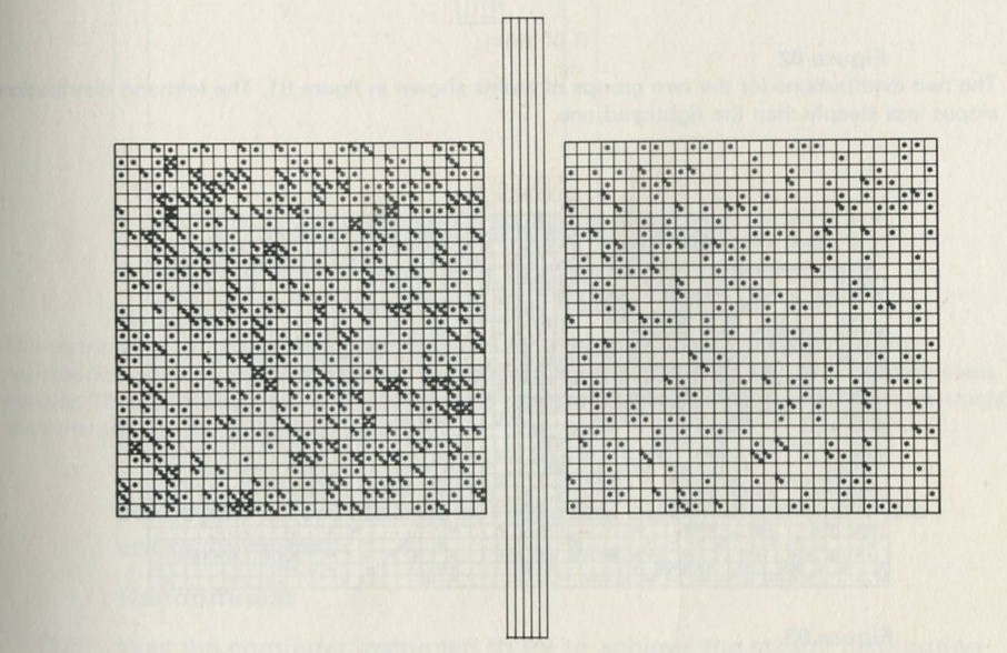
Figure 61: On the left, 900 quanta among 900 atoms. On the right, 300 quanta among 900 atoms. The two are not allowed to exchange energy, but quanta are being shuffled about within each one.
Full Size Image
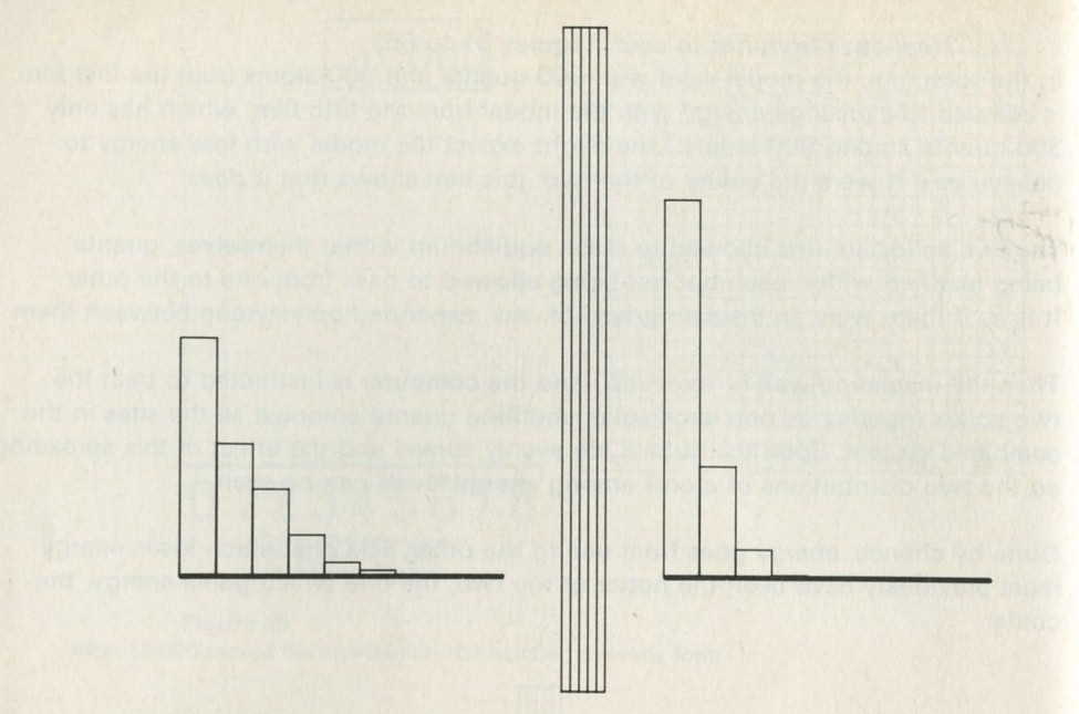
Figure 62: The two distributions for the two groups of atoms shown in figure 61. The lefthand distribution slopes less steeply than the righthand one.
Full Size Image
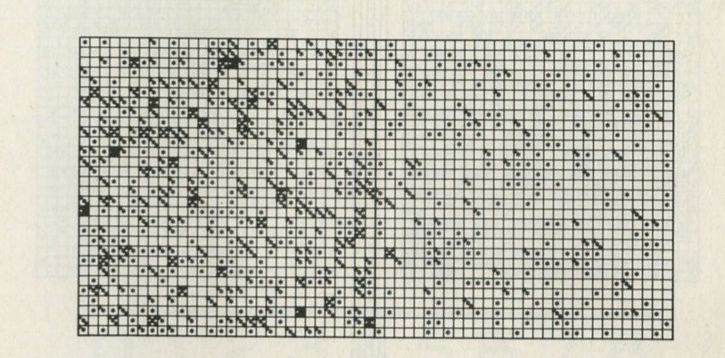
Figure 63: The two groups of atoms just as they are put 'in contact', but before any quanta have been moved about at random following this change.
Full Size Image
Figure 64: ... some time later! Quanta in the system shown in figure 63 have been allowed to move about at random, favouring moves from one group of atoms no more or less than moves from the other. But the quanta are now evenly spread between the two. After this, quanta still shift about, but there is no more overall change.
Full Size Image
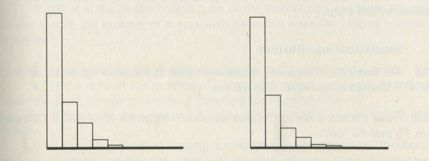
Figure 65: The distributions of atoms among energy levels for the system shown in figure 64, after equilibrium has been reached. The two distributions are essentially similar, sloping downwards equally. They both slope more steeply than the lefthand distribution in figure 62, but less steeply than the righthand distribution in figure 62.
Full Size Image
What can be learned about thermal equilibrium from the computer films?
Randomness
Q20 Was the computer instructed to try to achieve the steady distribution shown in figures 40, 41, 42, 47, and elsewhere? What was it told to do?
Q21 Would it have been possible in the first film, figures 34 to 42, to predict in advance the locations of atoms which would have no quanta at the 10 000th move?
Q22 In the sixth film, figures 61 to 65, was the computer instructed to move quanta from left to right rather than from right to left? What was it told to do?
Q23 In the 5000 moves from figure 40 to figure 41, is an atom with as many as seven quanta especially likely to lose one? Is an atom with no quanta especially likely to acquire one?
Q24 Look at figure 39.
- a Is one particular atom more likely to be chosen in the hundred and first move than any other atom?
- b Is it likely that the atom picked upon to lose a quantum will have just one quantum?
- c Is it likely that the atom chosen to gain one quantum will have just one already?
- d Is it likely that the hundred and first move will end up with one atom more with no quanta, one atom more with two quanta, and one atom fewer with one quantum?
- e Do the impartial random moves produce a definite trend in overall behaviour at this stage?
Statistical equilibrium
Q25 Are there about as many atoms with one quantum in figure 40 as in figure 41? Compare figures 45 and 46 too.
Q26 Have the same atoms got one quantum in figures 40 and 41? Compare figures 45 and 46 too.
Q27 Say in what sense there has been a change from figure 40 to figure 41.
Q28 Say in what sense there has been no change from figure 40 to figure 41.
Q29 Say in what sense the outcome of the different changes to the different starting points shown in figures 43 and 34 is, in the end, essentially the same. (See figures 41 and 46.)
Q30 In the computer film, did the distribution change in any way between the moments shown in figures 40 and 41 ? Did its general shape change?
Q31 Hard. Suppose that another time, a set of moves led back from figure 40 to figure 39 (the computer could be run backwards, perhaps). If the moves after that were random, what would you expect to happen? Why do you think no such backward run occurred in any of the films?
The shape of the equilibrium distribution
Questions 25 to 31 were about the fact that one definite distribution is ultimately reached by the game working itself out, wherever it starts off from. The following questions are about the shape of this distribution.
Q32 Look at figure 42.
- a What, approximately, is the ratio of the number of atoms with no quanta to the number with one quantum?
- b What, approximately, is the ratio of the number of atoms with one quantum to the number with two?
- c What, approximately, is the ratio of the number of atoms with two quanta to the number with three?
- d Give a general rule for the shape of the distribution.
- e In radioactive decay, if half the nuclei decay in time T, a further half will decay in a further time T. What is the.rule for the shape of the distribution of numbers decaying in successive equal time intervals? What is the name of the mathematical form of the process of radioactive decay?
- f What is the mathematical form of the distribution of atoms among energy levels; thatis. the number of atoms with particular energies plotted against those energies?
Q33 Look at figure 60, the distribution for the colder model solid.
- a Is the ratio of the number of atoms with a certain energy, to the number with one more energy quantum, a constant for this distribution?
- b Is this ratio the same as for figure 42, the hotter model solid? What is the ratio?
- c If there are N atoms sharing a total of q quanta, there are theoretical arguments which say that the ratios discussed in question 32 and in this question should be equal to (1+N/q). Test this prediction for figure 42 (N = 900, q = 900), for figure 60 (N = 900, q = 300), for figure 65 (N = 1800, q = 1200), and for figure 50 (N = 625, q = 625).
The theoretical reasons are outlined in Part Five, and given in more detail in Appendix B. Here you are merely making an experimental test of the answer they give. We shall use this answer at the end of Part Four to make a prediction about the heat capacity of solids.
Q34 In what sense is the distribution in figure 50 the same as that in figure 42? Why is it the same?
Heat going from hot to cold
Q35a Starting at figure 63, was the computer instructed to try to reach something like figure 64? What was it told to do?
Q35b In figure 63 the top lefthand atom has one quantum; in figure 64 it still has one quantum. In figure 63, the bottom lefthand atom has one quantum; in figure 64 it has no quanta. Could these results have been predicted in advance?
Q35c In figure 63 the atoms on the left share more quanta than those on the right. In figure 64, they share more nearly equal numbers. Could this change have been predicted in advance?
Q36a When the two halves of figure 63 are allowed to exchange quanta quite at random, there is a net flow of energy from left to right. Does such a flow occur from the part with a steeply sloping distribution to the part with a shallow or gently sloping distribution, or the other way round?
Q36b When a saucepan of soup is put on the plate of an electric cooker, does heat flow from high to low temperature, or the other way around?
Q36c After the stage shown in figure 64, quanta travel in equal numbers either way. Will the distributions shown in figure 65 change any more? How do they compare in terms of steepness?
Q36d If a casserole is put in an oven, when will its temperature stop rising and stay steady?
Q36e Which half of figure 63 is hotter? What about figure 64?
Q36f In questions 32 and 33 you thought about the ratio of the number of atoms with any particular energy to the number with one more quantum of energy. This ratio, being the same for all such pairs, describes the whole of a distribution by just one number. Steeply sloping distributions have a large ratio, shallow ones have a small ratio. Which go together, large ratio and high temperature (and small ratio and low temperature) or the other way around?
Part Four will conclude by showing how to fix upon a fundamental measurement of temperature, related to the distribution ratio.
The likely thing happens
Q37a Why, in a large school, is the number of people absent with colds almost constant from day to day (except during epidemics)?
Q37b Did the computer know that the equilibrium distributions should be exponential?
Q37c Is it fair to say that in each film, anything could happen, so what did happen was what was likely to happen?
Summary: chance and the flow of heat
If you have watched the computer films and thought about the questions related to them, you now have some reason to believe the following things.
Two lumps of solid of the same material (not in contact) which have the same proportion of internal energy to number of atoms will sooner or later, probably already, have the same distribution of atoms amongst possible energy levels, and the same temperature. (They had better not be compressed by different amounts - that would alter the energy levels.) It doesn't matter how they start off; they end up the same.
This will have come about by chance. In either lump, different atoms will be at different energies from time to time, but the relative numbers of atoms with different energies will stay remarkably steady, just because they are not made to do so, but are allowed to share energy at random.
Equilibrium is not static, in one sense, because the atoms continually exchange energy. However, it is steady, in that the equilibrium distribution, once reached, is permanent until outside conditions alter. But fluctuations around the average steady equilibrium distribution do occur, as chance tries out the possible variations on the arrangement of quanta among atoms.
The approach to equilibrium is definitely a one-way-only process. It comes about inexorably, but quite by chance, because what happens is what is likely to happen. If there are many atoms and quanta, what is likely to happen is so very, very likely that it always does happen in the end.
For the simple Einstein model solid, the equilibrium distribution is exponential in form. The distribution has a constant ratio of the number of atoms with one particular energy to the number of atoms with one quantum more energy. So atoms with no quanta are more common than atoms with many quanta. The distribution ratio is related to the number of atoms sharing each quantum. N atoms sharing q quanta have a distribution ratio of (1+N/q). (See question 33, or Part Five, or Appendix B.)
The distribution ratio is related to the temperature. Small ratios go with high temperatures; large ratios with low temperatures. The ratio and the temperature both become equal when two objects come together in thermal equilibrium. Temperature and distribution ratio both describe the object as a whole, summarizing its average behaviour. Each is a quantity that decides how likely it is that heat will flow one way or the other.
Heat goes from hot to cold in one way only, inexorably, but not because it is pushed. Heat flow occurs by chance, and happens because it is likely to happen. It happens inexorably because, with many atoms and quanta, it is very, very likely to happen.
The absolute Kelvin temperature scale
Note to teachers
It is suggested in the Introduction that some students might stop at the end of Part Four, though others may go on a little further. This brief piece about Kelvin temperature and the piece about the heat capacity of a solid which follows it are meant to round off Part Four for those who stop there. Part Five develops the same ideas in more detail, with less assertion. Those who are going on could pass straight from here to Part Five.
We decided that a high temperature goes with a low value of the ratio that describes the equilibrium distribution of the Einstein model solid. Now temperature ought to have a numerical value; we expect to be able to say that the temperature of something is, say, 300 K. How might distribution ratios be linked up with temperatures measured in kelvins, so as to go further than to be able vaguely to say that the temperature is high or low? This is what we now consider.
The temperature is related to the steepness of the distribution. Fixing the relation between them is mainly a matter of deciding how to relate them, not of discovering anything new. For we already know what hot means for the model: a small slope or ratio. It is just a matter of giving the right kind of number to the slope.
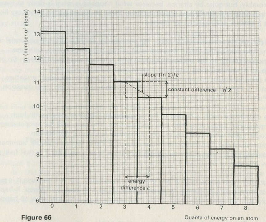
Figure 66: Logarithmic plot of the distribution of atoms among energy levels for an Einstein solid with 106 atoms sharing 106 quanta, each of size ε.
Full Size Image
Figure 66 illustrates a slightly different way of showing the slope of a distribution. It is drawn for an Einstein model with N = 106 atoms and q = 106 quanta, so that the ratio (1 + N/q) is equal to 2. (See question 33)
Unlike earlier distribution diagrams, the quantity plotted against the energy of an atom is the logarithm (base e) of the number of atoms with that energy, not simply the number itself.
A detailed calculation shows that we should expect 5 � 105 atoms with no quanta. ln(5 � 105) = 13.122. The number with one quantum will be half as many, 2.5 � 105. But ln(2.5 � 105) must simply be less than ln(55 � 105) by the amount ln 2. So the logarithmic distribution plot drops like a straight staircase, each step being equal to ln 2.
If we write ε for the energy of one quantum, the energy difference between levels, the slope of the logarithmic plot is simply (ln 2)/ε. In general, for N atoms and q quanta, the slope will be [ln(1 + N/q)]/ε.
Now the temperature T is high when the slope is small. So a reasonable decision would be to have T inversely proportional to the slope. With a constant k to turn the proportionality into an equality, we have:
kT = ε/ln(1 + N/q).
This is just a decision. We could have had T directly proportional to the slope, but then hot things would have low numerical values of 'temperature, which happens not to be normal practice. We could have had T inversely proportional to the square of the slope. That would merely be unnecessarily complicated.
Does this temperature T behave sensibly? If the solid acquires very many quanta, q becomes big and (1 + N/q) comes nearer and nearer to 1. So ln (1 + N/q) becomes nearly zero, and T goes off towards infinity. More and more energy makes the solid hotter and hotter.
Previously, we chose to make kT = ε/ln(1 + N/q). If we had used (1 + N/q) in place of its logarithm, which might seem simpler, the temperature would have had an upper limit. The sum of (1 + N/q) can never be less than one, so kT would have a largest value equal to ε. There would be an absolute hottest on such a temperature scale. That is why we did use the logarithm.
What about less energy? The solid cannot have fewer than no quanta, q = 0. Then both (1 + N/q) and ln(1 + N/q) become as big as one pleases, and the temperature T becomes zero. So this temperature T has the value zero at the point where the Einstein solid is as cold as it could ever be.
So T behaves sensibly, and has its zero at the absolute zero, that is, at the coldest imaginable condition.
A temperature T whose meaning is restricted to one very special model may not seem to be much use. But it happens that the definition can be generalized so as to cover any model involving particles distributed over energy levels, even if the levels are not equally spaced. So you may regard the explanation of how T can be interpreted in terms of a model of atoms and quanta as a simple example of a more general, but more complicated, interpretation. The essence of the idea is correct, but the details need attention in a fuller treatment.
Note to teachers kT= ε/ln(1 + N/q)
Appendix B, The Einstein model and the Kelvin temperature, discusses more fully the introduction of a temperature based on statistical ideas.
The equation given serves only for an Einstein solid. But it is a special case of an equation of quite general application. As shown in Part Five, ln(1 + N/q) is the change in the logarithm of the number of ways of arranging q quanta among N oscillators, when one more quantum of energy ε is added to the system.
Thus the equation can be written kT = ε/ Δ ln W, where W is the number of arrangements of quanta, and Δ ln W is the change corresponding to the addition of energy ε. This result is general, and may be applied to any material whatever. Usually it is hard to get a value for W or Δ ln W; the Einstein solid is of interest because calculating the value of Δ ln W is not too difficult.
The reason for introducing the energy ε into the equation is passed over in the treatment in Part Four, but a reason is given in Part Five and in Appendix B.
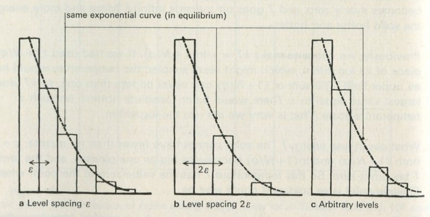
Figure 67: Equilibrium of materials with different level spacings.
Full Size Image
The reason is illustrated in figures 67 and 68. Figure 67a shows the distribution for an Einstein solid of level spacing ε. Figure 67b shows such a solid with level spacing 2ε. Figure 67c shows the distribution for a material with arbitrary level spacings. All have been drawn in the form which deeper theory predicts they will have if they are mutually in equilibrium. The quantity which is the same for all, and which so relates to their mutual temperature, is not the ratio between numbers of atoms in adjacent levels. The numbers of atoms in levels fit onto the same exponential curve if it is plotted on the same energy scale.
Figure 68 shows the corresponding logarithmic plots. The quantity that is the same for all three is the slope, which is the difference in the logarithms of numbers of atoms in adjacent levels divided by the level difference.
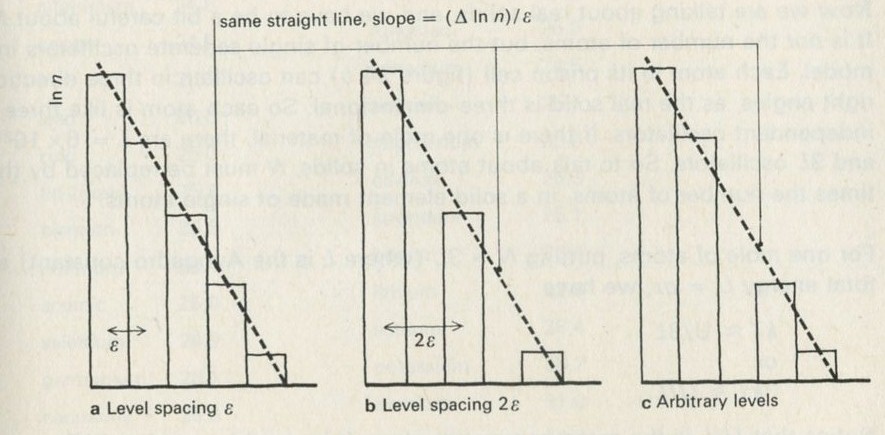
Figure 68: Logarithmic plots of the distributions shown in figure 67.
Full Size Image
The heat capacity of an Einstein solid
In the equation kT = ε/ln(1 + N/q), the quantity k was put in as a constant of proportionality. We shall now think about its meaning, and estimate its value by experiment.
We shall need one mathematical trick. Notice that for hot enough objects, the number of quanta is big compared to the number of atoms, so N/q is small. Now ln(1 + x) is nearly equal to x itself when x is small. Table 5 gives some values:
x     1+x   ln (1+x)
1.0   2.0   0.693
0.5   1.5   0.405
0.25  1.25  0.223
0.1   1.1   0.095
0.01  1.01  0.00995
Table 5
If the Einstein solid is hot enough, we can replace ln(1 + N/q) by N/q. Then the expression for T is very simple:
kT ≈ ε / (N/q) = qε/N
But qε is the number of quanta multiplied by the energy of a quantum, and is thus the total energy shared by the atoms, which we shall call U.
Now we are talking about real solids, and we have to be a bit careful about N. It is not the number of atoms, but the number of single separate oscillators in the model. Each atom in its prison cell (figure 24 b) can oscillate in three directions at right angles, as the real solid is three-dimensional. So each atom is like three independent oscillators. If there is one mole of material, there are L = 6 � 1023 atoms and 3L oscillators. So to talk about atoms in solids, N must be replaced by three times the number of atoms, in a solid element made of single atoms.
For one mole of atoms, putting N = 3L (where L is the Avogadro constant) and the total energy U = qε, we have
kT ≈ U/3L
or
3kT ≈ U/L
Notice that U/L is the mean energy per atom. It is roughly equal to 3kT.
Constant thermal capacity for many elements
The above result has a startling consequence. Suppose one mole of atoms of a solid element is warmed up, rising in temperature by ΔT, its energy U rising by ΔU, then
3k ΔT ≈ ΔU/L
or
3kL ≈ ΔU/ΔT
But ΔU/ΔT is the heat capacity of one mole of the element; the energy delivered to raise the temperature one degree (at fixed volume). The argument above says that the molar heat capacities of all solid, monatomic elements at high enough temperatures will all be the same, always supposing that the Einstein model is good enough to describe them. For the quantity 3kL is the same for all elements, L being the Avogadro constant and k the constant of proportionality we put into the equation defining temperature.
Table 6 gives some heat capacities for one mole of some elements.
Iodine is included to remind you that molecules arranged in a solid will take up more energy, because (among other things) the molecule can vibrate within itself as well as vibrating as a whole. Of the monatomic solid elements, a great number have very similar molar heat capacities, running at about 25 J mol-1 K-1, which is striking confirmation of the general correctness of the prediction.
Element   Cp/J mol-1 K-1   Element   Cp/J mol-1 K-1
carbon:                    gold        25.2
1 diamond    6.06
2 graphite   8.65          nickel      26.0
boron       12.0           cobalt      25.6
beryllium   17.8           manganese   26.3
silicon     19.8           chromium    23.3
aluminium   24.8           molybdenum  23.5
copper      24:5           tungsten    25.0
iron        25.2           vanadium    24.5
lead        26.8           titanium    25.1
zinc        25.0           magnesium   23.9
tin (grey)  25.8           calcium     26.3
bismuth     25.5           strontium   25.1
antimony    25.4           barium      26.4
arsenic     25.0           lithium     23.6
selenium    24.9           sodium      28.4
germanium   26.1           potassium   29.2
cadmium     25.9           caesium     31.0
silver      25.5           iodine (12) 55.0
(Cp is the heat capacity per mole at constant pressure. The value at constant volume, which should have been used, is too little different from Cp to matter. All values are given for temperature 298 K and pressure one atmosphere.)
Table 6 Molar heat capacities.
Dulong, Petit, Einstein, and heat capacities
This rule of constant heat capacities is not a new one. Dulong and Petit discovered it as a rough rule by studying heat capacity data a very long time ago. It was used by chemists to help settle atomic masses.
It is not a completely general rule. At low temperatures, q is not large and N/q is not small, so that the approximation to the logarithm of 1 + N/q fails. The effect is that the heat capacity drops to lower values. Just how hot an element must be for q to be much larger than N depends on the energy level spacing ε. (A few large-sized quanta represent as much energy as many smaller ones.) In table 6, the elements like carbon, for which the heat capacity is less than about 25 J mol-1 K-1, are those for which the quanta are large, and relatively few in number. They do not really spoil the story, for it is found that at higher temperatures, their heat capacities do rise to the value given by Dulong's and Petit's rule.
Einstein actually invented his model to try to explain how and why the heat capacities do fall off at low temperatures. To do so is not very hard: one simply does the (harder) calculation of ΔU/ ΔT without making the approximation ln(1 + N/q) ≈ N/q. The agreement with experimental data is then good, though not perfect, over a wide range of temperatures.
Note to teachers
It would be unfair to claim the prediction of Dulonq's and Petit's rule as a great success for the Einstein model, pleasing as it is. For it is very insensitive to the assumptions that go into the model used to predict it. It is given by a classical argument which assigns average equal energy �kT to each degree of freedom. Each oscillator has two degrees of freedom - kinetic and potential energy terms - and each atom is equivalent to three oscillators.
The Einstein model also gives the rule correctly. Its success was rather in predicting, for the first time, the form of departures from the rule. Other models, in which the energy is carried about by elastic waves, also yield the rule, and are better than Einstein's at getting the form of departures from it correct. Current research aims to improve the agreement between theory and experiment by making more detailed and realistic calculations based on the motions of interacting sets of atoms, and by allowing, for example, for the effects of non-linearity in the displacement-force law, and so on.
Value of the Boltzmann constant k and mean energy per atom
It seems reasonable that the roughly constant value 25 J mol-1 K-1 is a fair estimate of the quantity 3kL predicted for the molar heat capacity of one-atom solid elements by the Einstein model.
3kL = 25 J mol-1 K-1
but L = 6 � 1023 mol-1
so k=1.39 � 1023 JK-1
The value given in data books is
k = 1.380 � 10-23 JK-1
k is called the Boltzmann constant. We have presented it as a scale constant. introduced so that temperature T is measured on a particular scale.
In measuring the heat capacities, the temperatures were measured on the usual scale with about 273 one-degree intervals between absolute zero and the temperature of melting ice. The measurement of k must be in joules per kelvin units if T is in kelvins, so that kT is in joules, although k could be chosen to be any size whatever. But the value of k settles the scale of T. If k has the value above, T is in kelvins, and the scale of T is called the absolute Kelvin scale.
Since U/L ≈ 3kT (at high enough temperatures) and U/L is simply the mean energy per atom, we can say that the temperature T is roughly proportional to the mean energy per atom. This is not an exact result, but it is a useful one.
Also, kT has the order of magnitude of the mean energy per atom. At room temperature, 300 K, the value is of the order of 4 � 10-21 J. It reaches one electronvolt, 1.6 � 10-19 J, at about 10 000 K.
Physicists like to remember that kT is of the order of the mean energy per atom. They like it so much that they sometimes forget that it is only an approximate result, and that the temperature is not exactly proportional to the mean energy per atom.
You should also be able to remember a similar result in the kinetic theory of gases. There, too, the mean energy per molecule is proportional to the temperature, and is roughly equal to kT.
Note to teachers
Mean energy per atom
Appendix B, The Einstein model and the Kelvin temperature shows that of two materials, it is quite possible for the one with the lower mean energy per atom to be the hotter. However, for one material, it will be true that if the temperature rises, so does the mean energy per atom.
Kinetic theory of gases
See the introduction to this Unit, and the Teachers' handbook. The kinetic theory ought to be shown to all students at some stage. As it is fully discussed in the Nuffield O-level programme, we arrive at similar ideas at Advanced level by a different route, using solids.
But if students took a different O-level course, and missed the theory, it must be fitted in now, and an appropriate sacrifice of other material must be made. The rest of this Unit could be one such sacrifice.
See, for textbook material for students:
Rogers, Physics for the inquiring mind, Chapters 25 and 30.
PSSC. College physics, Chapter 20; Physics, Chapter 9.
Nuffield Physics Special, Molecules and motion.
Experiment: 9.9 Measuring the Boltzmann constant k
This hardly counts as an experiment: you may have done it before, you know what will happen, and you know the answer. But it may help to remind you how the ideas fit together.
You just have to measure how much energy ΔU is needed to warm an aluminium block by a measured temperature rise ΔT. Then k is given by
k ΔT ≈ U/3 � (number of atoms).
Find the mass of the block and calculate how many atoms of aluminium it contains. The energy can be delivered and measured electrically.
Calculate ΔU divided by three times the number of atoms; the rise in mean energy per oscillator in the Einstein model. As this rises, more oscillators fill high energy levels and fewer occupy low levels. The distribution becomes less steep, which is to say that the aluminium is hotter. Indeed, a little energy goes at once to the thermometer, just as energy flowed from the hotter, less steeply sloped distribution to the cooler, more steeply sloped distribution in the sixth part (Heat goes from hot to cold) of the Change and chance film. The thermometer rises because the aluminium's distribution has shifted.
The thermometer is marked in Kelvin-sized degrees (though the markings are probably Celsius degrees.) These degrees have an arbitrarily decided size: 273 of them from absolute zero to the ice point, and 100 of them from ice to boiling water.
The constant k links arbitrarily-sized Kelvin degrees with shifts in distributions of oscillating atoms in energy levels, which is the basis of our fundamental idea of temperature. We understand by k the mean rise in energy per oscillator divided by the change in Kelvin temperature (as long as the temperature is high enough).
Experiment: 9.9 Measuring the Boltzmann constant k
77 aluminium block
75 immersion heater
542 thermometer ( -10 to 110�C)
507 stop watch or stop clock
1003/5 ammeter (10 A)
1004/3 voltmeter (100 V)
or
1005 multi-range meter (25 V)
42 lever arm balance
59 l.t. variable voltage supply (d.c.)
and
1064 low voltage smoothing unit
or
176 12 volt battery
1000 leads
The aluminium block has a large hole drilled in it to take the heater, and a smaller hole tor the thermometer. A drop of oil in the thermometer hole helps thermal transfer. The ammeter and voltmeter are used to record the power delivered to the heater. The temperature rise is noted at its maximum, after a few minutes heating. In essence, the experiment is an electrical measurement of the heat capacity of the aluminium block.
The Boltzmann factor
We have introduced the temperature as a measure of how gently an exponential distribution slopes. Thus, at high temperatures, there will be proportionately more atoms in high energy levels, having many quanta, than at low temperatures. This fact can now be expressed quantitatively.
The factor (1 + N/q) is the constant ratio between numbers of atoms in adjacent energy levels. If nlow is the number in the lower level, nhigh is the number in the higher level, and the levels differ by energy ε,
nlow/nhigh = (1 + N/q)
But from the previous way in which temperature was introduced,
ln(1 +N/q) = ε/kT.
Thus ln(nlow/nhigh) = ε/kT.
so that (nlow/nhigh) = eε/kT
When T is small, ε/kT is large, and eε/kT is yet larger, so that there are many more atoms in the low level compared to those in the higher level.
The ratios of numbers of atoms in any pair of levels is also obtainable, since the ratio is the same for each adjacent pair of levels. The factor eε/kT just becomes eε/kT � eε/kT � eε/kT.... = eε+ε+ε.../KT, each level having eε/kT times more atoms than the next. Thus, for any pair of levels different by energy E,
nlow/nhigh = eE/kT
or, since it is often more interesting to know how many high energy atoms there are,
nhigh/nlow = 1/eE/kT
which is
nhigh/nlow = e-E/kT
The factor e-E/kT is called the Boltzmann factor. Its importance is that its use is not restricted to simplified situations like Einstein solids, but is valid for most sorts of materials. In Part Six, it will be used to study processes that depend on those atoms or molecules which have particularly high energies, such as those which evaporate from wet clothes on a washing line, or those which are able to take part in chemical reactions.
Summary of Part Four
In the Summary: chance and the flow of heat, we set out the ideas to be learned about thermal equilibrium from the study of the model of a solid, using the random games and computer-made films. You should look at this again.
Since then we have introduced temperature into the argument. Before, we saw that heat goes from hot to cold because that is the likely thing to happen. To say that one thing is hotter than another is just to say that energy is likely to flow from the hotter one to the colder one. It is so very likely that it happens as inexorably as gases diffuse and mix (or as tidy desks become untidy).
Temperature is a number related to how likely it is that energy will flow from one thing to another. Here this is partly concealed, but Part Five brings it out into the open. If you stop at Part Four, just remember that the temperature describes the distribution of atoms among energy levels. If there are a high proportion of atoms with large energy, the temperature is high. And an object with such a gradually sloping distribution readily loses energy to another object with a steeper distribution slope, which has fewer atoms in high energy levels.
Sooner or later, objects in contact come to equilibrium. When they have, their temperatures are equal. They are equally likely to pass energy one way as the other. Their distributions have equalized, so that the relative numbers of atoms in levels different by the same energy are identical.
A high temperature does not push heat from hot to cold. The flow happens by the chance, random, sharing out of energy among atoms. The temperature is an indicator of how likely it is that a body will, on balance, lose or acquire energy in this random shuffling process.
A place to stop
You could stop here, if you have had enough. Part Five goes on to develop the idea of temperature and the chance of heat flow more quantitatively. Part Six contains a number of important applications of the ideas, to engines, to chemistry, to pressures of vapours and electric currents in some materials, and to other matters. It reaches the great Second Law of Thermodynamics, and the idea of entropy.
But what you have done may seem enough. Even the Second Law is there, for it may be expressed in the form, heat flow, left to itself, always goes from hot to cold. You already know why this is so, and that is no mean thing.
5. Counting ways
Note to teachers
This Part contains difficult arguments, rather densely packed together. It may be that some students should miss it out completely. But the results reached are so far reaching in scope, and so deep in their importance, that we hope that some at least will try the work.
The whole Part should therefore be regarded as optional. It may be worth trying it to see how it goes, being ready to abandon it if the going is sticky. There is about a week available for Parts Five and Six, so the work here is not worth attempting if it would take more than a few lessons.
An overall view of the argument
This Part is wholly theoretical, devoted to developing further the understanding of the exchange and interchange of energy in a material, upon which a beginning was made in Part Four.
In earlier Parts we saw that what happens by chance is what happens in many ways; so to begin with, we inquire about the number of ways in which quanta of energy can be rearranged amongst the oscillators of the Einstein model described in Part Four. Because what matters in thermal equilibrium is the exchange of energy between two objects, we shall ask by how much the number of ways changes when energy is added or taken away. It turns out that the answer to this question is simpler than the answer to the question about how many ways there are of sharing quanta overall: indeed you have already met it as the factor (1 + N/q). in Part Four.
Then we argue that the exponential shape of the equilibrium distribution revealed in the computer experiments of Part Four can be explained in terms of this factor.
But the shape is related to the Kelvin temperature, and it is then possible to relate the temperature to the change in the number of ways of rearranging quanta when energy is added or removed, thus giving a fundamental relationship between temperature, energy, and counting of ways.
Finally, a new quantity, the entropy, is introduced. It is seen as a device for counting ways or changes in numbers of ways, without actually having to do the counting. It does this by exploiting the relationship between between temperature, energy, and numbers of ways referred to above.
As is appropriate to the more rigorous arguments given here, we shall refer to the sites in the Einstein model as oscillators. One atom, which can oscillate in three perpendicular directions, is equivalent to three such oscillator sites.
Counting ways of sharing quanta in an Einstein solid
When chance is the arbiter, what happens often is what happens in many ways. In Part Four, we have seen that when quanta are allowed to rearrange themselves at random amongst the oscillators of an Einstein solid, they find a steady, equilibrium distribution which has an exponential form, and also that quanta will sometimes go spontaneously from one such solid to another. We have seen that the meaning of hot and cold can be related to this random shuffling of quanta among atoms. To go further, it seems sensible to try to put these ideas together. To begin with, we try to see what counting the number of ways in which the quanta can arrange themselves among oscillators would be like.
Figure 69 shows an Einstein solid with just two oscillators - not a plausible thing in real life, but one that is easy to think about. It is shown with differing numbers of quanta shared amongst these oscillators.
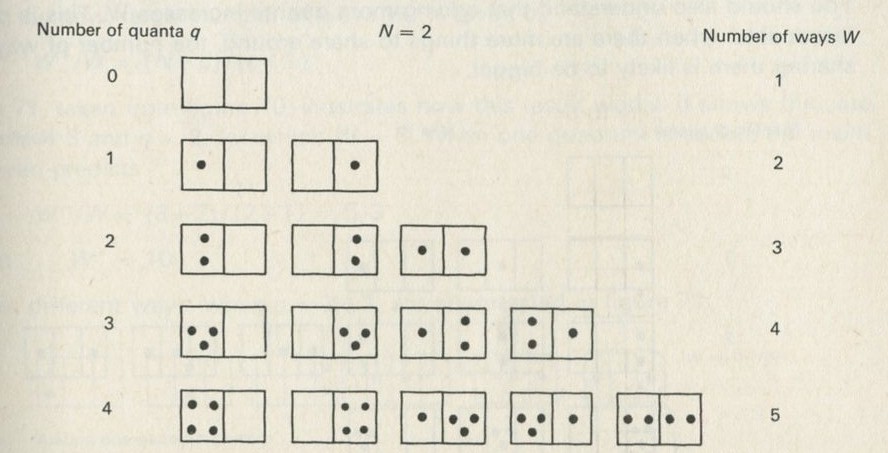
Figure 69: A two-oscillator Einstein solid
Full Size Image
Clearly, from figure 69, when the number of oscillators N = 2, the number of ways W of rearranging q quanta is simply q+ 1. The value of W is never so simple if there are more oscillators, but three features remain the same:
1 The number of ways can be counted by systematically rearranging the quanta in all possible arrangements, W being the number of such rearrangements.
2 The larger the number of quanta, the larger the number of rearrangements.
3 There is only one way of sharing no quanta.
Figure 70 illustrates the difference that is made by having three oscillators instead of two. For any given number of quanta, the number of ways W of sharing them is larger, but W still increases for every extra quantum, and its least value is still 1.
It is possible to work out a general result for W in terms of q and N. Doing this is not very hard, but is a distraction from our main purpose. The result is
W= (N+q-1)!/(N-1)!q!
For those who would like to see how the deduction goes, it is given in Appendix B in which the meaning of the symbol ! is given. But what really matters is that you understand what the job of finding W involves: simply counting out all the possible rearrangements of quanta.
Substituting N = 3 and q = 3 in the general result gives W = 10, as it must, as figure 70 shows. If there are many atoms and many quanta, W is very large; for example, for 900 oscillators and 900 quanta, as in several of the computer experiments of Part Four, W is about 10540. Obviously, such a large number is not to be discovered by actual counting, but must be deduced by argument.
You should also understand that adding more quanta increases W. This is pretty reasonable: when there are more things to share around, the number of ways of sharing them is likely to be bigger.
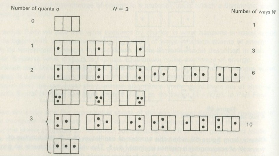
Figure 70: A three-oscillator Einstein solid
Full Size Image
Adding energy leads to more ways of sharing it
Boiling a kettle means getting energy to go from the hot-plate to the kettle. Firing an explosive charge means getting energy to go violently into warming up the surroundings, at the expense of the chemicals in the charge. Making hydrogen and oxygen from water means getting energy from somewhere to break the hydrogen-oxygen bonds. Making a petrol engine work means getting energy from fuel combinations, and then from hot gases, to go into the kinetic energy of a moving car.
All the interesting and useful processes which involve energy involve getting it to go from one thing to another. It is not surprising, then, that what matters more than the number of ways of sharing energy out in a material, is the change in the number of ways when energy is added or removed.
As before, we continue to think about the special case of the Einstein solid, because it is reasonably easy to think about. Some, though not all, of the answers are applicable in general: this is what makes the exercise worth the bother.
We start by giving a result for the effect on the number of ways W of adding one quantum to an Einstein solid. This result, proved in Appendix B, comes from the result for W itself mentioned previously. As will be seen, the computer films also give evidence that this new result for the effect of adding one quantum is right.
If there are N oscillators sharing q quanta in W ways, and one more quantum is added, the new, larger number of ways W* is given by
W*/W= (N+q)/(q+1)
Figure 71, taken from figure 70, illustrates how this result works. It shows the case where N = 3 and q = 2, for which W = 6. When one quantum is added, the result just given predicts
W*/W= (3+2)/(2+1) = 5/3
so that W*=10
The ten different ways, when q = 2+ 1, are enumerated in figure 71.
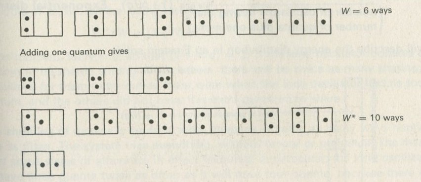
Figure 71
Full Size Image
The factor (1 + N/q)
Suppose there are 1 000 000 quanta shared among 1 000 000 oscillators. If one quantum is added, the number of ways goes from W to the larger value W*, where
W* /W = 2 000 000/1 000 001 ≈ 2 000 000/1 000 000 = 2
Now recall that N and q are, for decent-sized lumps of matter, going to be in excess of 1020, and it is clear that the factor (N+q)/(q+1) can be written as (N+q)/q, that is (1 + N/q), without making any appreciable error.
This is our first main theoretical result. When one quantum is added to an Einstein solid consisting of N oscillators sharing q quanta, the number of ways W increases to W*, where
W*/W = (1 + N/q) ......Result 1
It contains the similar result for the effect of taking away one quantum, for this is like going from the system with W* arrangements to one with W arrangements. Taking one quantum away has the effect of dividing W by the factor (1 + N/q).
In Part Four, the factor (1 + N/q) was guessed to be the ratio of numbers of oscillators with energies different by one quantum, in the exponential equilibrium distribution of an Einstein solid (figure 72). We shall now inquire how it comes about that the distribution is exponential, having just this ratio. We shall argue that it follows from result 1 above, that the exponential distribution,
(number of oscillators having any particular number of quanta) / (number of oscillators having that number of quanta plus one more) = (1 + N/q), Exponential distribution
will describe the energy distribution in an Einstein solid.
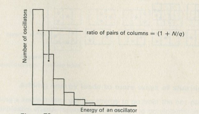
Figure 72
Full Size Image
One oscillator competing with many others for energy
We now think about one oscillator, exchanging quanta with a whole large collection of other oscillators, as illustrated in figure 73.
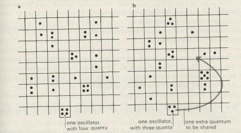
Figure 73
Full Size Image
Suppose, to be definite, that this one oscillator has four quanta. If, at some other time, it has only three quanta, the spare quantum is now available to be shared among the others. If the collection of many oscillators contains a very large number, N, of oscillators, sharing a very large number, q, of quanta, adding one more quantum increases the number of ways in which quanta can be arranged amongst them from W to W*, where, using result 1,
W*/W= (1+N/q).
For the moment, let N = q, so that (1 + N/q) = 2. If the lone oscillator donates one quantum to be shared among all the others, there will be twice as many sharing possibilities for them to try out as there were when the lone oscillator had its fourth quantum, and the others did not have this extra quantum to share.
If the shuffling of quanta is random, what happens in twice as many ways happens twice as often. The system tries everything, without favour or prejudice. The result is that some states of affairs are in effect favoured: in particular, the lone oscillator will have three quanta twice as often as it will have four quanta, because there are twice as many arrangements with an extra quantum shared amongst the collection of many oscillators, as there are with an extra quantum not so shared.
The situation is similar to several of those discussed in Part Three. A card drawn from a pack is more often not an ace than it is an ace, because there are more ways to draw a card which is not an ace. Shaken boxes of marbles are more often found mixed than sorted, not because sorted arrangements are avoided, but because there are fewer of them than there are of unsorted arrangements.
In general, because, using Result 1,
(number of ways of sharing any particular number of quanta) / (number of ways of sharing one fewer quantum) = (1 + N/q), it follows that, for any one oscillator sharing quanta with many others, (number of occasions when an oscillator has any particular number of quanta) / (number of occasions when it has that number of quanta plus one more ) = (1 + N/q) .... Result 2
Result 2 is nearly, but not quite, what we require. It says how often just one oscillator has each of two different energies. To explain the exponential distribution, we must be able to say how many oscillators have each of two energies, at one moment. An argument linking these two questions follows.
The biography of an oscillator: what happens often to one happens to many
In the fourth film in the series, Change and chance; a model of thermal equilibrium in a solid, illustrated in figures 51 to 56, the fate of just one oscillator was followed over a long period of time. Instead of looking at the behaviour of many oscillators at one time, the biography of one of them was examined.
A subtle and difficult argument
No one can blame you if you find the foregoing argument hard to follow. It is subtle, and it is difficult. It is, we believe, right in essence, but a full, careful, and complete argument would be even harder to follow. Such an argument is to be found in the most advanced books of statistical mechanics, under the title, the canonical ensemble.
If you find it too much to cope with, it may be best to take the following more general view. The experiments in the computer films suggest that the equilibrium distribution for an Einstein solid has the ratio (1 + N/q), in that the suggestion that this is the ratio can be tested against the results of the experiments. The computer is, in effect, being used to show what happens, as an alternative to having to calculate it. It is also easy to see that the ratio (1 + N/q) has a simple meaning. It is the ratio we have called W*/W, the ratio of numbers of ways of arranging quanta after and before adding an extra quantum. The exponential distribution having this ratio arises because any one atom has to share quanta with the rest, and the average behaviour will be decided by the relative numbers of ways there are of sharing or of not sharing extra quanta.
Justifying statistical arguments
Teachers will rightly be concerned that we are relying heavily on the results of a game which is far from obviously correct. The game gives the right answer because it has been carefully designed to do so. It is offered to students as something they can see and do, which shows the behaviour that can be predicted by rather arduous mathematics. Perhaps they will think it a fairly plausible guess. It can only be justified (or otherwise) by results.
A more formal approach does not escape this kind of difficulty, but has to rely on basic assumptions that are far from obviously true. Instead of supposing that a game may be adequate, a formal approach develops further the counting of ways of sharing. It then makes the unobvious assumption that all ways are equally likely, and this assumption too is only to be justified by results.
Boltzmann himself discovered which kind of ways to treat as equally probable by picking the kind that gave the right answers. We need not be too depressed if our game was developed in the same way.
It can, however, be proved that the game ought to yield an exponential distribution (for large N and q). See Appendix C, The quantum shuffling game for indistinguishable quanta.
The flow of heat from hot to cold
Why does heat go from hot to cold? If the answer were not rather interesting, the question would seem a silly one. The interest of the answer lies not so much in its content as in what kind of answer it is. It is not an answer of the kind, Because it is pushed ..., or of the kind, It must because this causes that ..., such as one might give to a question about why a spacecraft moves more quickly as it comes nearer to the Earth. The answer is of the kind we have given before in this Unit, but not elsewhere in the course. (However, in Unit 1, it could have been argued that a rubber band has the length it has because that is the most likely length.) Heat flow from hot to cold happens by chance; it happens because it is likely to happen. It always happens because it is so very, very likely to happen that the chance of its not happening is too remote to bother about.
The sixth film in the series, Change and chance: a model of thermal equilibrium in a solid, illustrated in figures 61 to 65, gives an example of what this answer means, and the idea is summarized in Part Four.
It is now possible to discuss this example more quantitatively. The lefthand half of figure 61 has 900 oscillators and 900 quanta. (For atoms in the captions, now read oscillators) If it were to lose one quantum, the number of ways of sharing quanta within that half would be divided by two (the ratio 1 + N/q, with N = q). In fact, W for this half goes from about 10540 to half that number.
The model solid on the righthand side of figure 61 has only 300 quanta shared among 900 oscillators, so that (1 + N/q) = 4. The 300 quanta can be rearranged in some 10300 ways, as it happens, but if an extra quantum is added to their number. W is multiplied by four.
When the two parts are separate, as in figure 61, any of the 10540 ways of arranging quanta in the lefthand part can co-exist with every one of the 10300 ways for the righthand part. The total number of ways for both at once is the product of these two. or 10840.
Now suppose that they are put in contact, as in figure 63, and that one quantum goes from left to right. The new total number of ways is the product of the two new numbers of ways for each part, given above, and is thus given by
new number of ways = � � 10540 � 4 � 10300
= 2 � 10840 compared with 10840 ways beforehand.
The transfer of a quantum makes more difference to the number of ways for the cold part than it does for the hot part. The net effect of a transfer from left to right is an increase in the number of ways, so such transfers will happen more often than not. Further quanta will be likely to follow the first, until a further transfer does not any longer increase the number of ways.
Certainly, quanta do go the wrong way. Such a move reduces the number of ways, in this example by a factor 2 (W for the righthand part being divided by 4, W for the lefthand part being multiplied by 2). So to start with, the impartial effect of chance will be to make transfers from left to right four times as often as from right to left. But this is another way of saying that quanta will, on average, go the proper way. Would 50 quanta go the wrong way? This would lead to a reduction in the number of ways of 250 times, compared with an increase of 250 times for flow the right way. So the first is 2100 times more likely than the second. Similarly, that 50 quanta should flow the right way is about 250 times more likely, and that they should flow the wrong way is about 250 times less likely, than is no net flow. It is this one-way transfer that makes us call the one half hot and the other cold.
The general meaning of hot and cold
Looking at figures 63 and 64 you might well feel that we have been to a great deal of trouble to discuss a simple matter: that energy goes, like scent in a room, from where it is more concentrated to where it is not. This is, in fact, a quite proper objection: the effect shown in figures 63 and 64 is little different from diffusion. But heat flow is not always just like diffusion, for in general, materials exchanging heat will not be as simple as the Einstein solid model. Their energy levels need not be equally spaced, and they need not be identical materials. We have tried to cast the argument in a form which illustrates a general rule about heat flow, whose value is not limited to special simple models.
For any pair of objects whatever, if the thermal transfer of energy raises the number of ways in which the atoms can be distributed over energy levels (more crudely, the number of ways of sharing the energy out amongst the atoms), then such a transfer Will happen. A cold object is always one for which there is a large effect on the number of ways, when energy flows in or out. A hot object is always one for which the corresponding effect is small. Two objects are in thermal equilibrium if taking energy from either and giving it to the other reduces the number of ways for the first by the same factor as it increases the number of ways for the second.
Hot means good energy giver because fewer quanta lead to not too many fewer ways.
Cold means good energy taker because more quanta lead to very msany more ways.
Equally hot means exchanging quanta has the same effect on the number of ways.
Temperature and changes to number of ways
The temperature can be given a quite precise expression in terms of changes to numbers of ways.
For the Einstein solid, we saw that the addition of one quantum multiplied the number of ways by a factor, and we have now seen that this factor depends only on how hot the solid is. Let the factor have any value, say 1.5.
Then W*/W = 1.5
if one quantum is added. If another quantum is added, and W* now means the number of ways after adding both quanta,
W*/W = 1.5 � 1.5.
If many quanta are added, the result is the long product of factors
W*/W = 1.5 � 1.5 � 1.5 � 1.5 ....
It is convenient to take logarithms, and it is conventional to use natural logarithms, to base e. Then if W* is the number of ways after adding many quanta,
In W*/W = ln W* - ln W = ln 1.5 + ln 1.5 + ln 1.5 + ....
so long as the added quanta amount to too little energy to make a significant difference to the ratio (that is, to how hot the solid is).
On the righthand side of this equation giving the change in ln W, there are just as many terms equal to ln 1.5 as there are quanta added, so the righthand side is proportional to the change ΔU in the energy U shared among the atoms of the solid, since ΔU is the number of added quanta multiplied by the energy of each quantum. (The energy U could be changed in other ways, for example, by squashing the solid, but we are restricting ourselves to changes in U brought about by adding quanta, that is, by promoting some atoms to higher energies while keeping the same set of levels.)
Writing Δ ln W for the difference ln W* - ln W, we obtain
Δ ln W ∝ ΔU (constant volume, almost constant temperature)
The interest of this result is that it is not restricted to the simple case of the Einstein solid, but can be applied to most sorts of matter, solid, liquid, or gas.
Previously, we saw that high temperatures T go with small changes in numbers of ways. Clearly, Δ ln W cannot be proportional to T, for that would have the reverse effect. In order to settle on a way of relating temperature to numbers of ways, the conventional choice is to put
Δ ln W ∝ ΔU/T (constant volume, nearly constant temperature)
This is a matter of choice; we are trying to find a fundamental way of expressing an idea which so far has been given no quantitative meaning (apart from arbitrary practical scales) - the idea of temperature. To have 1 /T2 in place of 1/T would be permissible, but foolish, since it would only complicate matters for no good reason.
The proportionality of Δ ln W to ΔU/T can be made into an equality by inserting a constant k, giving
Δ ln W = ΔU/kT
or kT = ΔU/Δ ln W (both at constant volume, and for small changes)
This is our second main result; a fundamental definition of temperature in terms of energy and numbers of ways. The name Boltzmann constant has been given to k.
Kelvin temperature and the Boltzmann constant k
The next step is to consider what meaning and value to give to k. If we choose its value arbitrarily, then the scale of temperature is settled, as the following example shows. The simplest arbitrary value to give to k is 1. Think now of a typical Einstein solid, to which one quantum is added. In the instances so far, the ratio W*/W = (1 + N/q) has been between 1 and 10, so Δ ln W is a number of the order 1. ΔU is here the energy of one quantum. If the frequency f of atomic oscillations is of the order of 1012 Hz, which is about right, the energy of a quantum (hf) is of the order of 10-21 joule per quantum, h being the Planck constant. Then kT is also of the order of 10-21 joule per particle, and if k = 1, T is of the order 10-21 joule per particle.
It may seem odd to have temperatures whose values are always minute and are in joules per particle. From an atomic point of view, this could be thought to be very natural, since T is, simply, roughly equal to the average energy one atom possesses.
Despite the naturalness of this way of looking at temperature, the custom is to have temperatures measured on another scale, on which values of T are larger and more convenient. Instead of choosing the value of k, the usual thing to do is to choose to measure T in units, and on a scale, of its own, and to find what value of k that choice implies. It should already be clear that if T is a number greater than 1, k must be very small, because kT is very small.
The convention is to decide, quite arbitrarily, that the temperature of melting ice is just 273 degrees above absolute zero. This scale is called the Kelvin scale, and temperatures are measured in kelvins, symbol K. Room temperature is about 300 K, for example, while helium is a liquid at about 4 K. Because kT is in joules, k will now have the unit joules per kelvin, symbol J K-1.
Triple point
Strictly, the choice on which the Kelvin scale is based is that the triple point of pure water, at which solid, liquid, and vapour phases are in equilibrium, has the temperature 273.16 K. The melting point of ice at atmospheric pressure is then 273.15 K.
In order to measure the value of k which follows from choosing the Kelvin scale for T, one has to find some physical system - anything will do - for which the change Δln W can be calculated when energy ΔU is added. There are many ways of doing this job. One way, using a gas as the material whose change in numbers of ways is calculated, appears in Part Six. Because we already know how to calculate Δln W for an Einstein solid, it is convenient at this stage to use that model again.
Measurment of k: the Einstein solid as a means of counting ways
For an Einstein solid, with q quanta shared among N oscillators, the ratio W*/W = (1 +N/q), for one quantum added, so that
Δln W = ln(1 +N/q) (addition of one quantum)
If one quantum of energy ε is added, the energy U of the solid increases by ΔU = ε.
Then the equation
kT = ΔU / Δ ln W
which defines the temperature T, becomes
kT = ε/ln(1 +N/q).
In Part Four, this same equation was produced, though T was there defined in a less fundamental way, as relating to the slope of an exponential distribution.
In Part Five, we have seen how the slope of the distribution is related to changes in numbers of ways.
Starting in Part Four, at The heat capacity of an Einstein solid, there was given an argument which led from the equation above - relating temperature T to the energy levels and numbers of atoms and quanta - to the result
molar heat capacity of an Einstein solid ≈ 3 kL
where L is the Avogadro constant. This result was seen to be an approximation which might be expected to be good at high temperatures, but not at low temperatures. If you omitted the argument in Part Four, you can go back to it now.
Table 6 in Part Four gives values of molar heat capacities. The table makes it clear that, as predicted there is a group of solid monatomic elements whose heat capacities are all much the same. The value of this common heat capacity seems to be about 25 J mol-1 K-1.
Assuming that 3KL = 25 J mol-1 K-1
and since L = 6 � 1023 mol-1
then k= 1.39 � 10-23 J K-1
compared with k = 1.38 � 10-23 J K-1, taken from tables of physical constants.
You will notice that k is small, as we suggested it must be when introducing it in the previous section. k is of the order 10-23 J K-1 because at temperatures of the order 300 K, the energy one atom is likely to have is about kT. Since this energy is a few times 10-21 J, k = kT/T is of order 10-23 J K-1. The Boltzmann constant k can be regarded as a scale constant, ensuring that the numbers Δ ln W , or the small magnitudes of quantum energies, do not lead to very small numerical values of the temperature.
The Boltsmann factor
We can now bring out more of the meaning of the Boltzmann factor, first introduced in Part Four. This factor gives the ratio of the number of atoms to be expected in a high energy level to the number to be expected in a low energy level, if the levels differ by energy E.
It has its origin in the equation
Δ ln W = ΔU/kT (constant volume)
Just as in figure 73, and in the argument that goes with it, to promote one atom to a level having energy E above its present level, energy E must be taken from all the other atoms of the material and its surroundings, of which the one atom forms a part. This reduces the number of ways in which the energy can be shared amongst these atoms, by an amount given by
Where -E has been written for ΔU, since U is to be reduced by an amount E.
If W* is the number of ways after energy E is removed, and W is the number of ways before, then
ln W*/W= -E/kT
and W*/W= e-E/kT
But what happens in few ways W*, will happen rarely. The number nhigh of atoms which happen to acquire energy E will compare with the number nlow which do not, in the ratio
nhigh/nlow = W*/W so that
nhigh/nlow = e-E/kT
This is the result we reached in Part Four, arguing only in terms of the simple Einstein model. It has a wide range of applications, in physics and in chemistry, some of which are looked at in Part Six.
Counting ways with heaters and thermometers: entropy
Suppose you warm a kettle of water by 10 K, starting at room temperature (about 300 K). By what factor does the number of ways of spreading the energy over molecules rise, as a result of the added energy? The answer can be found from
Δ ln W = ΔU/kT(constant volume)
One kilogramme of water needs 4200 J to warm it by 1 K, so the kettle might have been supplied with 42 000 J, if it contained 1 kg of water. k ≈ 1 .4 � 10-23 J K-1, so we have
Δ ln W ≈ 42000/(1.4 � 10-23 � 300) ≈ 1025.
And this is only the logarithm of the number of times there are more ways after supplying the energy, compared with the number before. Since
ln(Wwarm/Wcool) ≈ 1025
Wwarm/Wcool ≈ e1025 .
Are we serious? Indeed we are: knowing Boltzmann's constant, it is possible to calculate changes in numbers of ways simply from measurements made with heaters and thermometers. Given such information, it becomes possible to begin to tackle some of the problems raised earlier in this Unit: problems about which way processes will go. Some of these applications are touched on in Part Six.
In the equation
k Δ ln W = ΔU/T (constant volume)
the quantity k Δ ln W on the left can be measured by means of measurements of the quantities ΔU and T, on the right. All that one requires is a heater and a thermometer which measures T in kelvins. In the above example,
k Δ ln W
has the value 42000/300= 140 J K-1.
The quantity k Δ ln W, which, unlike W itself, can be related directly to simple laboratory measurements in the way just described, has been given a special name. the change of entropy, written ΔS. Above, ΔS was 140 J K-1. In general,
ΔS = k Δ ln W
and, with a proper choice of the zero of S,
S = k ln W
This last equation seems only to be giving a new name to something introduced before. Yet it is the cornerstone of thermodynamics, from the statistical point of view. It says what entropy is. What is entropy? It is just the logarithm of the number W of distinct states a thing can be in, scaled down by the constant k to make the value more manageable. The result is important because entropy is a remarkably useful quantity to know about.
The meaning and use of entropy are discussed further in Part Six, where we see how entropy is measured, and how it is used by physicists, chemists, and engineers. Here we have merely introduced its definition in terms of W; a definition Boltzmann thought so important that he asked for it to be carved on his tombstone. Because every system tries out all the ways open to it, if more ways become accessible, it explores them all. W therefore tends to increase. If W increases, so does the entropy, k ln W. The rule that the direction of a process will be such as to increase the total entropy is called the Second Law of Thermodynamics.
Some qualifications, mainly for teachers
Entropy and thermodynamic parameters
For a change at constant volume V, the entropy change is given by
ΔS = ΔU/T
where U is the internal energy because, at constant volume,
ΔU/T= k Δ ln W.
At constant pressure P, a system can expand against the external pressure and the entropy change is now given by
ΔS = ΔH/T
where H, the enthalpy, is equal to U + PV so that, at constant pressure,
ΔH= ΔU + PΔV.
In general, the internal energy or the enthalpy can be increased by allowing a system to exchange heat Q with its surroundings. If this is done reversibly, then
ΔS = Q/T (reversibly).
The importance of the qualification reversibly is seen in the case of a gas which is allowed to spread into an empty space after a partition in its container is broken. The entropy increases, but if the gas is ideal, ΔU, ΔH, and Q are all zero. The increase in entropy can be found by achieving the same net change in a reversible way, here by an isothermal expansion. If the change is reversible, the entropy change Q/T of the heat sink is equal and opposite to the entropy change of the gas, the net entropy change of gas plus sink being zero in a reversible change. This is the idea which lies behind the use of a gas to measure the Boltzmann constant in example 1 in Part Six.
The equation kT = ΔU/Δ ln W
A more careful version of this equation would read
kT= [∂u/∂(ln W)]V
where the subscript V indicates that the volume is constant. When the volume is constant, the change in U, the internal energy, is equal to the heat Q exchanged reversibly with the surroundings and also to the first term in the sum
∂U = Σi εi ∂ni + Σini ∂εi.
Here εi are the energies of the levels of the system, and ni the numbers of particles in those levels. The first term represents an energy change arising solely from promoting or demoting particles amongst the various levels, the levels being kept the same. The second term represents the effect of shifts in the levels themselves. If the volume is constant, the levels do not shift. and the second term is zero.
In its careful form, the equation is of general application, since k d(ln W) = dS, the change of entropy, so that it can read
T= [∂U/∂S]V
which is the definition of temperature in terms of thermodynamic parameters.
The Boltzmann factor nhigh/nlow = e-E/kT
This result applies generally to all materials for which classical statistics are a good enough approximation. Strictly, therefore, it applies to nothing, since the statistics are always either Bose-Einstein or Fermi-Dirac, but in practice, the approximation to Maxwell-Boltzmann statistics is a good one except near absolute zero, or for such systems as electrons in metals, even at room temperature.
Note that the factor gives the relative populations of a pair of quantum states. Because there may, or may not be, many levels at or near to the selected pair, the factor is only a part of the whole calculation of the mean energy of a system, or of the number of atoms to be expected within any given small range of energy.
For example, in an ideal gas, the quantum states are not equally spaced along an energy axis, for there are many more states clustered within a fixed band of energy at high energies than there are at low energies. This arises because the states are essentially those of standing waves in a three-dimensional box, and there are many more standing waves of short wavelength than there are of long wavelength, within comparable small ranges of particle energy. Towards low energies, despite the rising trend of the exponential variation of populations within levels, the number of states available falls off sharply, and the actual numbers of molecules in narrow bands of energy fall towards zero. Towards high energies, the rapidly falling trend of the exponential ensures that, although there are many states to populate, the numbers of molecules populating them are small, and the distribution again falls. In between, at moderate energies, it rises to a maximum, giving the well known humped Maxwell-Boltzmann distribution for the energies of gas molecules.
However, it is very often the case that molecules of exceptionally high energy are of interest, especially in chemical reactions. For such molecules, the Boltzmann factor is usually by far the most important term and other factors can be neglected, to a fair approximation.
The canonical ensemble
The arguments for the exponential distribution and for the Boltzmann factor rely on imagined exchanges of energy between a large, constant temperature assembly of particles, and a small system, which is here a single oscillator. It is crucial to the argument as given, that there is only one way for energy to be arranged on one oscillator in a definite state, since the number of ways for the whole system is the product of the number of ways for the large part and for the small part. This point is not, however, stressed in the text. If the small part of the system is a collection of atoms, the argument can still be made to work, but is much harder, since both numbers of ways must now be taken into account.
Difficult as the argument is, its outcome is simple. A large heat bath is unlikely to supply energy E by chance to a small system, because to do so reduces W. The chance of it doing so is given by the Boltzmann factor.
6. Uses of thermodynamic ideas
The law that entropy always increases - the Second Law of Thermodynamics - holds, I think, the supreme position among the laws of Nature. If someone points out to you that your pet theory of the Universe is in disagreement with Maxwell's equations - then so much the worse for Maxwell's equations. If it is found to be contradicted by observation - well, these experimentalists do bungle things sometimes. But if your theory is found to be against the Second Law of Thermodynamics I can give you no hope; there is nothing for it but to collapse in deepest humiliation. This exaltation of the Second Law is not unreasonable. There are other laws which we have strong reason to believe in, and we feel that a hypothesis which violates them is highly improbable; but the improbability is vague and does not confront us as a paralysing array of figures, whereas the chance against a breach of the Second Law (i.e. against a decrease of the random element) can be stated in figures which are overwhelming.
Sir Arthur Eddington (1928), Gifford lectures, 1927: The nature of the physical world. Cambridge University Press.
Examples of uses and applications of thermodynamic ideas
This Part contains a number of short, independent sections, each giving an example of a use of ideas developed in the rest of the Unit. The aim is to illustrate that these ideas have a very wide range of applications, in physics, in chemistry, and in engineering. Time is too short to allow each example to be developed in any great depth, or with any care for detail. In any case, to develop it in that way might defeat the main purpose at this stage, which is simply to allow students to see the broad sweep of problems encompassed, rather than to teach them exactly how any one problem is solved.
We suggest, therefore, that two of the following examples should be selected, according to the tastes and ability of the class. It may be that teachers will feel able to base a short talk on the other examples, enough to show the range of ideas involved. Such a summary should, in any case, introduce the Second Law at least in terms of the principle that W does not diminish in any spontaneous change, whether or not the quantity entropy (S = k ln W) is mentioned.
If Part Five is omitted, there may be up to a week available for this Part, but the choice of examples will be restricted, as explained below. If Part Five is tackled, all the examples become accessible, but except with the cleverest students, time will be very short.
Choice of examples
Examples 2, 3, and 4 can all be used without requiring previous work from Part Five of the Unit. It might be possible in the same circumstances to make something of examples 1 and 5, but these are mainly intended, with examples 6, 7, and 8, to follow work on Part Five.
Example 1 uses the value 2N, for the factor by which the number of ways of arranging particles in a box is increased when the volume is doubled, to provide another means of estimating the value of the Boltzmann constant in a laboratory experiment.
Example 2 uses the Boltzmann factor to indicate in a general way why the vapour pressure of water increases with temperature, and to relate the rate of increase with the energy needed to evaporate water molecules.
Example 3 uses the Boltzmann factor to discuss the influence of temperature on the rate of a chemical reaction. It offers some striking experiments and, as a valuable link with chemistry, deserves rather a high priority in the selection of examples.
Example 4 uses the Boltzmann factor to explain the rapid increase in electrical conduction of a semiconductor material, when the temperature rises. It offers an experiment every student can do.
Example 5 introduces entropy. The values of entropy for various substances are discussed, in an attempt to make this quantity seem like any other physical quantity to which one is already accustomed, such as energy or momentum. It could be of particular interest to chemists.
Example 6 follows up the introduction of entropy in example 5, by using it to show how, in general, one might predict or understand the direction of a chemical reaction. This example links closely with work done in Nuffield Advanced Chemistry, Topic 17.
Example 7 deals with the inefficiency of heat engines, arguing from the non-diminishing property of the total entropy to the necessary inefficiency of an engine, rather than, as is customary, in the other direction. Given earlier work, this should prove a rather easy example. It has value as a very practical and socially significant consequence of ideas in this Unit.
Example 8 discusses electric cells as energy converters and shows how the voltage of a cell will depend on temperature and on concentration. This example should be found to tie in quite closely with work on cell and half-cell reactions that is likely to have formed part of an Advanced chemistry course.
Example 1: Volume change of a gas and the Kelvin temperature
The air inside a bicycle pump will never, all by itself, be found in one half of the pump. Nothing prevents the molecules from happening to place themselves all in one half, but that they should all independently do so would be too great a coincidence.
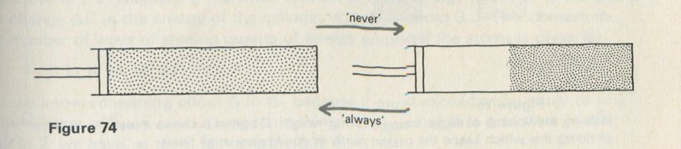
Figure 74
Full Size Image
Of all the ways of placing N molecules within the pump only one way in 2N ways has all of them in one particular half.
If the volume of a gas, which consists of molecules which move independently of one another and themselves occupy a negligible volume, is halved, the number of ways is divided by the enormous factor 2N, and we conclude that such a reduction will never occur.
But the volume of the air in a bicycle pump can easily be halved: one just has to push the piston in.
A weight placed on top of the piston will also do the job (figure 75) and the lowering of such a weight involves no change in numbers of ways. But if the process happens. it cannot be that, overall, the number of ways diminishes by a large factor like 2N.
When the experiment is tried (as if, absurdly, to check that it can be done) another feature is noticed. The gas or the cylinder becomes warmer, or both do. The energy transformed by pushing in the piston becomes spread out over the molecules of the gas and the cylinder. In addition to the decrease in number of ways by a factor 2N, we must reckon in the increase in the number of ways arising because this energy is now spread out over many molecules.
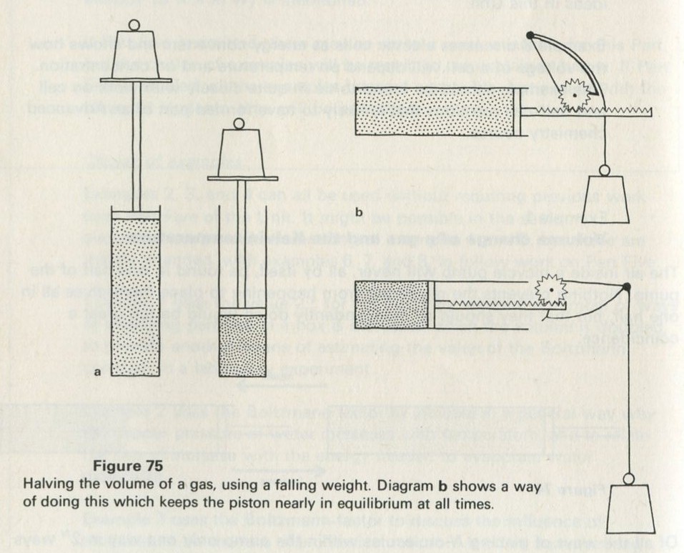
Figure 75: Halving the volume of a gas, using a falling weight. Diagram b shows a way of doing this which keeps the piston nearly in equilibrium at all times.
Full Size Image
If the piston is at each stage pushed just hard enough, but no harder, than is needed to compress the air in it a little more, the minutest reduction in the force on the piston would allow the gas to expand back a little. The process can be made two-way. If it can, there can be no overall change in the number of ways, for if there were the process would happen pretty well inexorably in one direction.
We shall consider one (not the only) means of achieving a two-way (the technical term is reversible) compression, which can be done in the laboratory.
The air is kept in an aluminium pump cylinder, and this cylinder has a much greater heat capacity than the air in it, so that this air is kept at an almost steady temperature, most of the energy transformed in compressing it going to the cylinder. A trial with an aluminium bicycle pump shows that the temperature change of the cylinder is indeed very small.
The energy transformed can be found in more than one way. It is possible to measure how much electrical energy is needed to warm the pump cylinder by the same amount as is observed when the air is compressed. It is also possible to calculate the energy transformed from the changes of pressure and volume, as in figure 76.
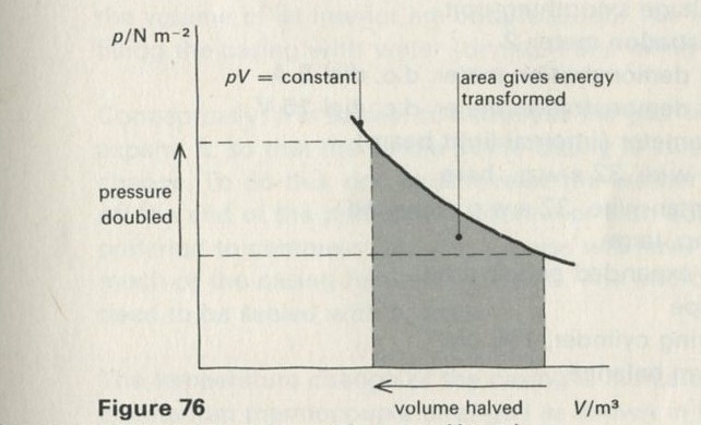
Figure 76: Calculation of energy transformed from a p-V graph.
Full Size Image
In one such experiment, in which the volume was halved, the energy transformed was close to 3 J. Neglecting the small amount of extra energy in the air in the pump, the change ΔU in the energy of the cylinder was thus about 3 J. The increase in the number of ways of sharing quanta of energy amongst the atoms is given by
Δ ln W = ΔU/kT.
But we know something about Δ ln W, because it must exceed or be equal to ln 2N, if the number of ways overall is not to diminish. Supposing that Δ ln W = ln 2N = N ln 2, we have, at room temperature 300 K,
N ln 2 = 3/300 k.
N is the number of molecules in the cylinder, which can be calculated from the Avogadro constant, knowing the volume of the cylinder. In the experiment being reported, N was 11 � 1020.
Using this value gives, for k
k= 1.3 � 10-23 J K-1.
The experiment is crude, but it illustrates how the Boltzmann constant can be found, using nothing more elaborate than a bicycle pump, employing a gas as a means of counting ways.
Demonstration 9.10: Boltzmann's constant and the behaviour of a gas
 1070  gas energy transfer apparatus
   77  aluminium block
   75  immersion heater
   59  l.t. variable voltage supply
 1064  low voltage smoothing unit
   70  demonstration meter 2
 71/2  dial for demonstration meter, d.c. dial 5 A
71/10  dial for demonstration meter, d.c. dial 15 V
 1001  galvanometer (internal light beam)
   2B  copper wire, 32 s.w.g., bare
 1054  constantan wire, 32 s.w.g., covered
 44/1  G-clamp, large
 1053  slab of expanded polystyrene
 1053  Sellotape
 1055  measuring cylinder, 100 cm3
   42  lever arm balance
 1000  leads
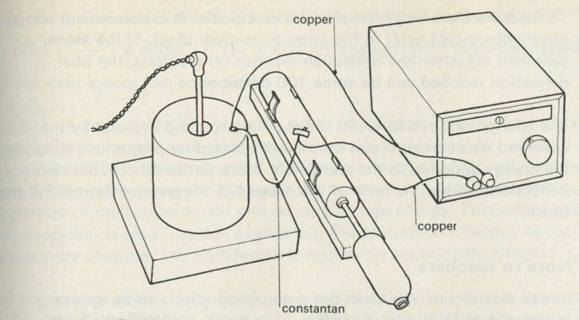
Figure 77: Boltzmann's constant and the volume change of a gas.
Full Size Image
A metal bicycle pump is used. An aluminium pump, whose heat capacity does not exceed 50 J K-1, is suitable. The mass of the pump casing and the volume of its interior are both required. The latter can be found by filling the casing with water (drying it and oiling it afterwards).
Conceptually, it is easiest to compress the gas. In practice, it is simpler to expand it, so that the whole of the casing is involved in the temperature change. To do this, one must reverse the washer on the piston, and seal off the end of the pump with a screw or with adhesive tape. If it is preferred to compress the gas, a guess will have to be made as to how much of the casing has been warmed. The end of the pump will then need to be sealed with a screw.
The temperature change of the casing is indicated by a copper-constantan thermocouple arranged as shown in figure 77. The � 1 range of the galvanometer is needed. A double junction couple, one junction being kept in a large heat sink (the aluminium block), is necessary. The piston is then pushed in (or pulled out) once, so as to halve (or double) the volume of the air. (If the volume ratio is not 2, but is f, the expression 2N just becomes fN.) The galvanometer should deflect by about two to four small divisions. It takes about 15 seconds for the full deflection to be attained.
A finger placed for a moment on the thermocouple produces a large deflection, indicating that the temperature change is very small, and also shows from the direction of the deflection whether the casing was warmed or cooled in the experiment. This test also makes it clear that the pump must not be handled anywhere but by the piston handle, when making the volume change.
To measure the energy transformed electrically, it is convenient simply to put an electrical heater in the large aluminium block. It the heater is switched oft when the deflection reaches 50 divisions, the final deflection reached will be some 100 divisions.
The energy required to warm the aluminium pump cylinder by the observed small amount can then be calculated by proportion, reducing the energy supplied to the aluminium block in the ratio of the two deflections and in the ratio of the masses of the pump cylinder and the block.
Note to teachers
In this experiment, the air in the pump undergoes a more or less isothermal, more or less reversible, change of volume. In an isothermal change, the internal energy of the gas is unaltered, all the energy transformed as work appearing as energy used to warm the surroundings very slightly. For the change to approximate to a reversible isothermal one, the piston must in principle be pushed with a force only infinitesimally larger than is needed to keep the volume constant.
In practice, the pump can be pushed in or out sharply. The surroundings of the gas must have so large a heat capacity that the temperature rise of the whole system is also infinitesimal.
PSSC, College physics, uses the equilibrium between an expanding gas and a heat sink as the major means of arriving at Δ ln W = Q/kT (where Q is the heat exchanged between gas and sink). The argument is given there very fully, though the entropy is given the non-standard meaning ln W rather than k ln W. See Chapter 22.
Example 2: The vapour pressure of water
How does one dry damp washing? It can be hung out on a windy day, or it can be warmed. Why does warming help? Because the water evaporates more easily, one might say. The Boltzmann factor e-E/kT turns out to be the main basis of this piece of common experience.
A molecule must acquire energy it it is to escape from liquid water. Part of this energy is needed to pull it away from other molecules, and part is needed to push back molecules in the air or vapour above the liquid. The energy needed can be measured by finding how much electrical energy is needed to evaporate a measured amount of water. The value per mole is ΔH ≈ 40 kJ mol-1. The energy per molecule is ΔH divided by the Avogadro constant, which is L = 6 � 1023 mol-1, so the energy per molecule ΔH/L ≈ 7 � 10-20 J.
At washing-line temperatures, say 300 K, the energy kT is about 4 � 10-21 joule, so the ratio (ΔH/L)/kT is about 17. (Actually, ΔH changes with temperature somewhat, but we shall ignore this correction.)
The Boltzmann factor e-E/kT gives the ratios of numbers of particles in two energy levels different by energy E. The extra energy per molecule ΔH/L is not a quantity exactly like E, but if the proportion of molecules with exceptionally high energy (here 17 times the energy kT) is small the factor e- (ΔH/L)/kT is quite a good guide to the proportion of molecules which will acquire a large energy. This works because the proportion is small, so that even when the proportion changes as the temperature changes, the numbers in lower levels are scarcely affected.
The importance of the factor lies in its great sensitivity to changes in temperature. At T = 300 K, the factor is about e-17. It takes only a small rise in temperature (to about 340 K) to turn the 17 into 15. But the factor e-15 is e2 ≈ 7 times larger than e-17, which means that this modest rise in temperature produces about 7 times as many molecules able to evaporate.
A fair guide to the number of molecules able to evaporate in a given time is the pressure p of vapour in equilibrium with the water. The ideas sketched here suggest, then, that p might vary with T in the form
p ∝ e- (ΔH/L)/kT.
In fact, the arguments we have used are very loose, and the variation has the general form
p = f(T) e -l!.H!L p = t(T) e- (ΔH/L)/kT,
but the function f(T) usually varies more slowly with temperature than the exponential term, so that over restricted ranges of temperature the exponential term is the one that matters. See Bent's, The Second Law, Chapter 33, for a treatment based on changes of entropy.
A simple way to measure the variation of vapour pressure with temperature is to use the fact that water will just boil at a temperature where the vapour pressure reaches the outside pressure on the water. If p varies in the way suggested, then,
ln p = - (ΔH/L)/kT + constant
Values of ln p plotted against 1/T would then give a straight line, as in figure 78. The slope should be -ΔH/kL, so the slope can be compared with ΔH/kL calculated from a measurement of ΔH. The experiment can be used to give an estimate of k.
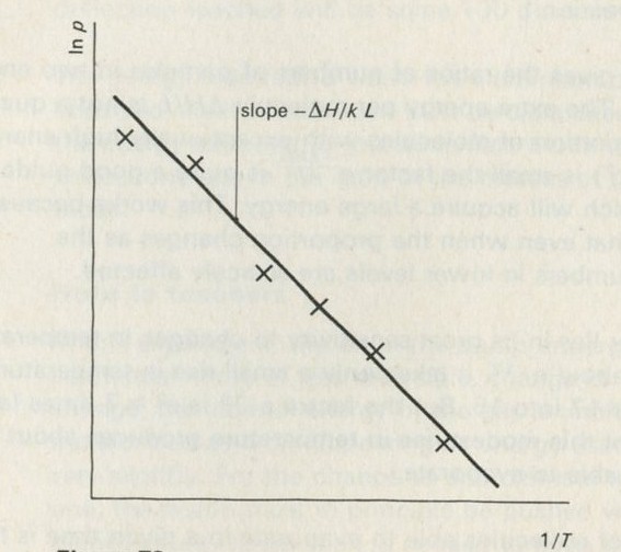
Figure 78
Full Size Image
Experiment: 9.11 The vapour pressure of water
9.11a Energy needed to evaporate water
1004/2 voltmeter (10 V)
or
179 d.c. voltmeter (0-15 V)
1003/5 ammeter (1 0 A)
176 12 volt battery
75 immersion heater (totally enclosed type)
1055 test-tube, hard glass, 150 � 25 mm
507 stop watch or stop clock
543 chinagraph pencil
1055 burette
1053 slab of expanded polystyrene with hole to take test-tube
1053 Sellotape
1000 leads
supply of boiling water
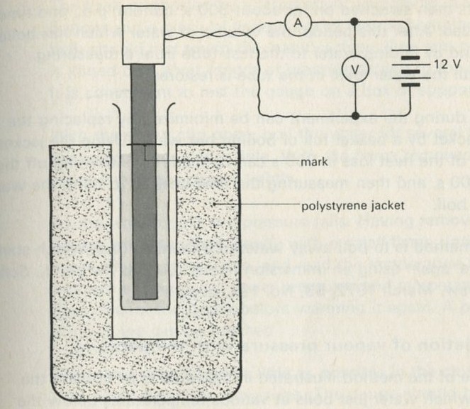
Figure 79: Electrical heater used to evaporate water.
Full Size Image
9.11b Variation of vapour pressure with temperature
67 Bourdon gauge
1054 rubber pressure tubing
548 round-bottomed flask (250 cm3)
542 thermometer ( -10 to 110�C)
1055 T-piece
1055 bung with 2 holes (for thermometer and T-piece)
522 Hoffmann clip
508 Bunsen burner
511 tripod
510 gauze
1054 piece of porous pot
503-6 retort stand base, rod, boss, and clamp
9.11b Energy needed to evaporate water
Any of the well-known means of measuring the energy needed to evaporate water will do. A simple, though rough, method is illustrated in figure 79. A test-tube, with an insulating jacket which may be a slab of expanded polystyrene with a cylindrical hole cut in it, has a 12 V immersion heater put in it. Hot water is poured in up to about 25 mm from the top of the tube, and is brought to the boil. After any water that was going to boil over has done so, the water level is marked with a wax pencil, with the heater switched off.
The heater is then switched on for about 300 s; current, p.d., and time being recorded. After this period, the volume of water which has boiled away is found by adding water to the test-tube from a measuring cylinder, until the water level in the tube is restored.
Heat losses during the experiment can be minimized by replacing the insulating jacket by a beaker full of boiling hot water. Using the jacket, an estimate of the heat loss in 300 s can be made by switching off the heater for 300 s, and then measuring the time needed to bring the water back to the boil.
A better method is to boil away water in a thermos flask which stands on a balance, again using an immersion heater. See Jarvis, W. H., School science review, March 1972, 53, No. 184, page 596.
9.11b Variation of vapour pressure with temperature
The principle of the method illustrated in figure 80 is to observe the pressure at which water just boils at various temperatures below the normal boiling point, using a pressure gauge connected to a flask in a sealed system with as little air in it as possible.
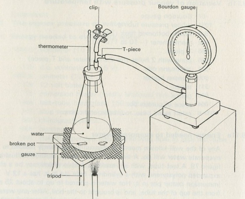
Figure 80
Full Size Image
The flask, supported by a retort stand and clamp, has a little water in the bottom and a piece of broken pot to reduce bumping. The thermometer bulb should just touch the water surface. One arm of the glass T-piece is joined by a short length of pressure tubing to the Bourdon gauge. It is convenient to rest the gauge on a box or support near the flask.
With the screw clip open, boil the water for several minutes to drive out as much air as possible. With the flame removed and when boiling stops, the clip is closed tightly.
As the water cools, the pressure falls. Having removed the tripod and gauze, warm the flask gently with a small flame until the water just boils again. Remove the flame, and read the temperature and pressure. This process is repeated at lower pressures and temperatures, by allowing the flask to cool for longer before warming it again. A pressure of about 1/4 atmosphere can be reached.
The water should boil as little as possible in the closed system, or a good deal could distill into the gauge. The gauge should be tapped before taking a reading.
Example 3: Rate of reaction
Why is it quicker to cook peas in a pressure cooker than in an open pan of boiling water? The reason has nothing directly to do with the pressure: it is that the water in a pressure cooker boils at a higher temperature (see example 2 if you want to know why} and peas cook more quickly at a higher temperature. A look at a pressure cooker recipe book will show you that the rate of cooking peas increases a great deal, taking perhaps a minute or two under pressure instead of the usual time of up to ten minutes. The rise in temperature that achieves this is not very big: at double atmospheric pressure (which is usual in pressure cookers), water boils at about 394 K instead of 373 K.
Another example of a change in the rate of reaction with temperature is the reaction between glucose and oxygen, catalysed by methylene blue. A sealed flask half full of colourless liquid is shaken, and then the liquid turns blue. The blue colour lasts for perhaps half a minute, and then the liquid becomes colourless again. The experiment can be repeated many times, with the same result.
If the flask is warmed by a few degrees, by being held in hot water, and is then shaken again, the blue colour lasts for a shorter time. The de-blueing reaction has happened more quickly.
Oxygen from the air in the flask rapidly converts colourless methylene blue into a blue oxidized form, when the flask is shaken. Then the blue methylene blue oxidizes glucose in a slow reaction, itself going back to the colourless form. The blue colour lasts until all the oxygen in transit is used up.
At first sight, one would expect a reaction not to be much affected by a modest rise in temperature. The number of molecular collisions per second will not increase as much as all that, as the temperature rises. If molecular energies vary in proportion to T, molecular velocities and so numbers of collisions per second might vary in proportion to √T, and therefore, doubling the absolute temperature would not even double the rate of reaction. In fact, the reaction rate will often double for a rise of only a few degrees in temperature.
The key lies in the Boltzmann factor e-E/kT Suppose that the reaction only occurs when a pair of molecules collide with unusually large energy. The Boltzmann factor gives the relative numbers of particles in energy levels different by energy E. If the number of molecules with unusually large energy is very small, the number in low levels will be nearly constant, even if the number of energetic molecules rises. In these circumstances, the proportion of molecules with large extra energy E is given adequately by the Boltzmann factor, so that we may expect the rate of reaction to vary as
rate of reaction ∝ e-E/kT
because the rate of the reaction is likely to be proportional to the number of molecules suitably equipped to react. The energy E is called the activation energy of the reaction. A large activation energy means a slow reaction, because few molecules are, at any moment, able to react.
The blueing-deblueing reaction can be studied quantitatively, but the time the blue colour lasts depends on how much oxygen is taken from the air in the shaking stage, and giving a flask a standard shake is not easy. Other reactions are available, and details follow.
One possible experiment involves the reaction of bisulphite ions and formaldehyde. The system is arranged so that the two substances, both colourless solutions, are mixed. The mixture remains colourless until all the bisulphite ions are used up, when a separate alarm clock reaction suddenly turns the mixture pink. The pair of solutions can be warmed before mixing them, so that the time t from mixing to the appearance of the pink signal can be recorded at various temperatures.
The rate of reaction is proportional to 1/t, so that we expect
ln(1/t) = -E/kT + constant.
A graph of ln(1/t) against 1/T, as in figure 81, should be a negative sloping straight line, and its slope yields an estimate of the activation energy per molecule.
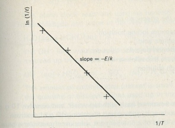
Figure 81: Plot of ln (rate of reaction) against 1/absolute temperature.
Demonstration or experiment: 9.12 Rate of reaction
9.12a Blue bottle
  1056    sodium hydroxide, 10 g
  1056    dextrose (glucose), 10 g
  1056    methylene blue 1 drop of 1% in ethanol
  1056    ethanol (ethyl alcohol)
  1055    flat-bottomed flask. 1 dm3 (1 litre)
   533    plastic bucket or basin
          supply of hot water
9.12b Formaldehyde clock
1056 sodium metabisulphite, 5 g
1056 sodium sulphite (anhydrous), 1 g
1056 formaldehyde, 10 cm3
1056 phenolphthalein, 20 cm3
1055 measuring cylinder, 100 cm3 2
512/1 beaker, 250 cm3 2 or more
517 volumetric flask 1 dm3 (1 litre) 2
542 thermometer ( -10 to 110�C)
507 stop watch or stop clock
533 plastic bucket or basin
supply of hot water
9.12c Iodine clock
As for b, replacing the chemicals by:
  1056   0.1 M potassium iodine solution
  1056   0.5 M sulphuric acid
  1056   0.1 M hydrogen peroxide solution
  1056   0.1 M sodium thiosulphate solution
  1056  0.2 % starch solution
9.12a Blue bottle
Half fill a 1 dm3 flat-bottomed flask with tap water, and dissolve 10 g of solid sodium hydroxide in it, adding and dissolving 10 g of dextrose afterwards. Add one drop of a one per cent solution of methylene blue in ethanol, and allow to stand until colourless. Seal the flask with a rubber bung.
Give the flask one or two vigorous shakes and the contents will turn blue. They will become colourless again after about half a minute or so, depending on how hard and for how long the flask was shaken.
Warm the contents of the flask by dipping it in hot water in a basin for a few minutes. A temperature rise of 5 to 10 K is plenty. When the flask is now given a standard shake, the blue colour lasts for a considerably shorter time.
The experiment is described at length in Campbell, Why do chemical reactions occur?.
9.12b Formaldehyde clock
Two solutions. A and B, are made up just before they are required (the shelf-life does not seem to exceed one day). Solution A is 5 g of sodium metabisulphite, and 1 g of anhydrous sodium sulphite, dissolved in water and made up to 1 dm3 in a volumetric flask. Solution B is 10 cm3 of formaldehyde and 20 cm3 of phenolphthalein, made up to 1 dm3 with water in a volumetric flask.
100 cm3 of each solution is measured out into pairs of beakers, and the contents of one of a pair of beakers are poured into the other at the moment when a stop clock is started. Before mixing some of the pairs, the beakers are stood in hot water for a short while, until their temperatures cover values over the range 20�C to 50�C. The temperature of the mixture is taken and recorded, together with the time taken for the mixture suddenly to develop a pink colour.
The main reaction is between bisulphite ions and formaldehyde:
HCHO(aq) + HSO3 -(aq) = CH2OHSO3 -(aq).
The alarm clock reactions used are twofold. Sulphite ions react with formaldehyde and water in the very slow reaction:
H2O(aq) + HCHO(aq) + SO3 --(aq) = CH2OHSO3 - (aq) + OH-(aq).
The OH- ions would turn the phenolphthalein pink, were they not mopped up by bisulphite ions in the fast reaction:
OH-(aq) + HSO3 -(aq) = SO3 - -(aq) + H2O(aq).
The amount of sulphite ions present is small, and the reaction is slow, so the quantity of bisulphite ions used up in these reactions is relatively unimportant. But when the main reaction has exhausted the bisulphite ions, the OH- ions are no longer removed, and the phenolphthalein indicator turns pink, signalling the end of the bisulphite-formaldehyde reaction indirectly.
The quantities need to be measured out with some care. Reducing the proportion of solution A in the mixture increases the time by about 1 s per 1 cm3 less than 100 cm3 mixed with 100 cm3 of B, at 20�C. The pink colour takes an appreciable time to develop, perhaps 2 s in a reaction time of 60 s. The reaction time varies from about 100 s at 15�C to 5 s at about 50�C, the rate doubling about every 10�C.
See Science masters' book (1964) Series IV, Part 2, Chemistry, page 230, John Murray.
9.12c Iodine clock
This is an alternative to the formaldehyde clock, the experiment being done in the same way. The reaction is between hydrogen peroxide and iodide ions, the end of the reaction being signalled by starch; this detects the presence of iodine which has used up all of a small amount of sodium thiosulphate added to the solution. Full details are given in Nuffield Advanced Chemistry Teachers' guide II, experiment 14.2. The details concern an investigation of the effect of concentration, but the experiment is suitable for an investigation of the effect of temperature in the range 15�C to 40�C, at one concentration.
Non-equilibrium arguments
It is surprising that it is possible to say anything about reaction rates, when the Boltzmann factor applies only to equilibrium situations. In effect, the excited, activated state is treated as if it were in equilibrium, which it is not. Therefore, the predictions made often fail to come true.
Example 4: Conduction in a semiconductor
When hot water is poured onto a thermistor which is connected to a battery and an ammeter, the current rises dramatically. Making the thermistor a little warmer makes it conduct a great deal better.
The key to understanding why this happens is the Boltzmann factor, e-E/kT. Very nearly all the atoms in a pure semiconductor have their electrons tightly bound to them, and the material would be like any other insulator except that the energy needed to excite an atom so that an electron is freed is not so great. Rarely, an occasional atom can acquire enough energy at the expense of the rest to become ionized, so the material conducts electricity a little.
The Boltzmann factor gives the ratio of the number of particles in energy levels different by energy E. As long as the number of atoms with energy large enough to become ionized is small, so that changes in this number make little difference to the numbers in lower energy states, the Boltzmann factor is quite a good guide to the proportion of atoms which will acquire, by chance, a large extra energy E.
If this explanation is along the right lines, because the current conducted will tend to be proportional to the number of free carriers, one might expect the current I to vary as
I ∝ e-E/kT
or
ln I = -E/kT + constant.
Note to teachers
A glance at any book about semiconduction will reveal that the above story is much oversimplified, though the basic feature, that the conduction depends on thermal activation of a few electrons, is correct. This is the feature we wish to emphasize.
Among the simplifications are the following. The energy levels belong to the crystal structure as a whole, falling into bands. In a pure semiconductor, the band of levels for electrons associated with conduction is of the order of one electron volt above the top of the band of valence electron levels. If the gap between the bands is E, a fraction eE/kT of electrons in valence levels will be promoted to the conduction band resulting in one conduction electron and a postive hole in the valence band. In effect, the energy per carrier is E/2, and this is the quantity for which the experiment will yield an estimate.
A doped semiconductor, as in transistor materials, is another matter. This contains impurity atoms which are much more easily ionized, and at low temperatures most of the conduction is due to carriers from impurity atoms. As the temperature rises, the conduction by carriers from impurity atoms, nearly all of which are already ionized, diminishes rather than increases, because the carriers become less mobile. At higher temperatures, the conduction due to electrons from the semiconductor atoms can overtake impurity conduction, as the number of electrons crossing the valence band-conduction band gap increases.
In the argument that the current would be proportional to the number of carriers, the effect of a rising temperature in reducing the mobility of the carriers was ignored.
The current passed by a thermistor at various temperatures can be measured, and a plot of ln I against 1/T might, on the argument given, be expected to be a straight line. The energy E needed for an atom to give rise to conducting carriers can be estimated from the slope of the graph, as in figure 82.
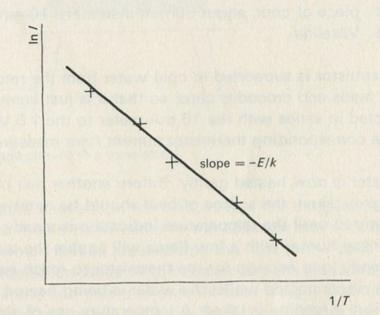
Figure 82: Variation in current passed by a thermistor, with temperature.
Experiment: 9.13 Change of current with temperature
132N thermistor (RS Components Ltd TH3)
1033 cell holder with one U2 cell
1003/2 milliammeter (10 mA)
1003/3 milliammeter (100 mA)
52K crocodile clip 2
542 thermometer ( - 10 to 110�C)
512/1 beaker. 250 cm3
511 tripod
510 gauze
508 Bunsen burner
503-6 retort stand base, rod, boss, and clamp
1000 leads
Alternative: add
1051 germanium transistor (e.g. QC 71)
1053 piece of cork, about 30 mm diameter � 10 mm thick
1053 Vaseline
The thermistor is supported in cold water from the retort stand by means of two leads and crocodile clips, so that it is just immersed, and it is connected in series with the 10 mA meter to the 1.5 V cell. Temperature and the corresponding thermistor current I are measured.
The water is now heated gently. Before another pair of corresponding readings is taken, the source of heat should be removed and the water stirred until the temperature indication is steady. Judicious use of the Bunsen burner with a low flame will enable the temperature to be kept steady long enough for the thermistor to reach equilibrium. The cell may be disconnected whilst the water is being heated. and reconnected just before a reading is taken. A temperature rise of about 10�C between readings is suitable.
A graph of ln I against 1/T is very nearly linear. In a typical experiment, the gradient E/k was found to be 4.1 � 103 K giving E = 5.6 � 10-20 J (0.35 electronvolt).
Alternative experiment with a transistor
The leakage current in a germanium transistor, between collector and emitter, can be used as a substitute for the current in a thermistor.
Figure 83 shows a way of mounting the transistor in a piece of cork, so that the transistor is immersed but its leads are clear of the water.
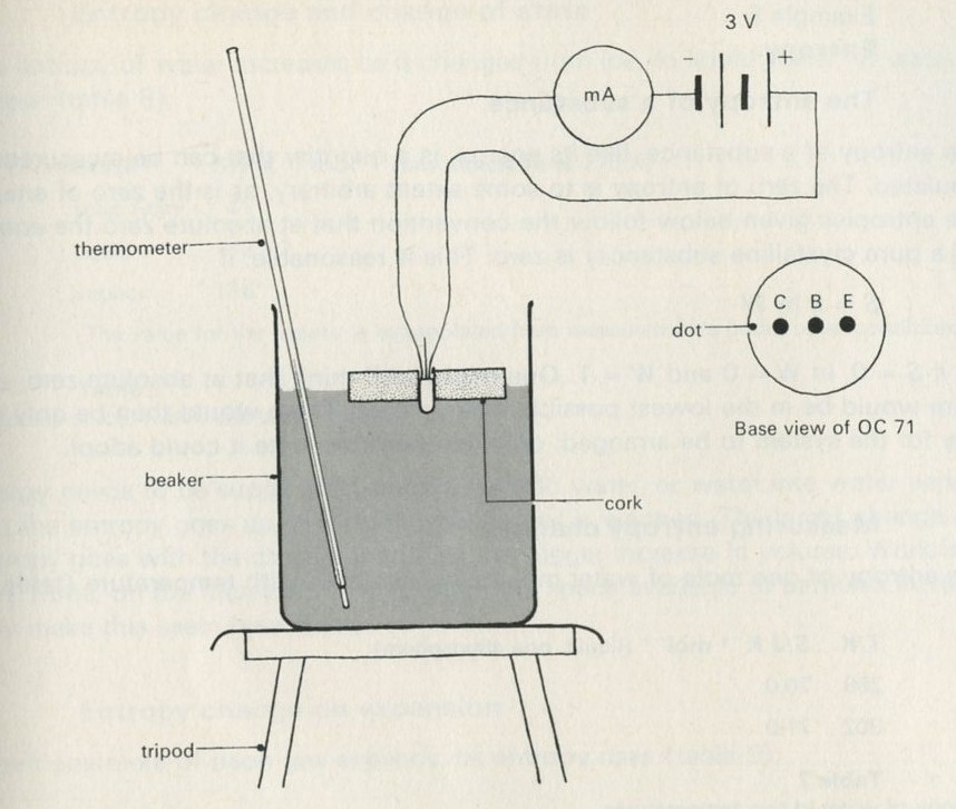
Figure 83: Measurement of leakage current in a transistor.
Full Size Image
A hole should be made in the cork so that the transistor is a tight fit in it. Light leads should be soldered to the collector and emitter leads of the transistor which is then pressed into the hole in the cork. The cork is carefully floated on water in the beaker and the leads are suspended from the retort stand and clamp to prevent their weight from tilting the cork. It is important not to get the leads from the transistor wet, and Vaseline can be put over them to prevent this.
It is essential to connect the collector and emitter with the correct polarity - the collector of a pnp transistor such as the OC 71 being connected to the negative side of the 3 V supply.
The temperature may be raised to about 45�C. When readings are taken, the temperature needs to be raised slowly and held steady until the transistor reaches equilibrium. This can be achieved by careful use of the Bunsen burner with a low flame. Readings should be taken at intervals of about 5�C. A 100 �A meter will be needed for temperatures below about 25�C.
Example 5: Entropy: The entropy of a substance
The entropy of a substance, like its energy, is a quantity that can be measured and tabulated. The zero of entropy is to some extent arbitrary, as is the zero of energy. The entropies given below follow the convention that at absolute zero the entropy (of a pure crystalline substance) is zero. This is reasonable, if
S= k ln W
for if S = 0, ln W = 0 and W = 1. One might well think that at absolute zero, every atom would be in the lowest possible energy state. There would then be only one way for the system to be arranged; only one possible state it could adopt.
Measuring entropy changes
The entropy of one mole of water molecules increases with temperature (table 7).
   T/K   S/J K-1 mol-1 (liquid, one atmosphere)
   298   70.0
   302   71.0
Table 7: Entropy of water at two temperatures.
Adding energy means that W (for the water) increases; more energy can be shared out in more ways. The increase in entropy ΔS = k Δ ln W can be measured, as was indicated in Part Five, by measuring the rise in energy of the material at a measured temperature. At constant volume, for example,
ΔS= ΔU/T.
(If the entropy change over a wide range of temperature is needed, the total change is the sum - or integral - of many such terms, T entering each term with the value it had at each stage.)
For example, 1 kg of water needs about 4180 J to raise its temperature by 1 K. To warm one mole of water (18 g) by the 4 K interval from 298 K to 302 K, just about 300 J are therefore necessary.
The entropy change, since the average temperature is 300 K, is given by
ΔS ≈ 300/300 = 1 J K-1 mol-1
and this is just the difference between the two tabulated entropies.
Entropy change and change of state
The entropy of water increases as it changes from ice, to liquid water, to water vapour (table 8).
   State      S/J K-1 mol-1 (one atmosphere, 273 K)
   solid (ice) 41
   liquid      63
   vapour     185*
(The value for the vapour is extrapolated from measurements under other conditions.)
Table 8: Entropies of ice, water, and water vapour.
Energy needs to be supplied to change ice into water, or water into water vapour, and the entropy goes up as it does when water is warmed. The larger change of entropy goes with the change involving the bigger increase in volume. Work in Part Three, on the increase in ways when the space available to particles increases, may make this seem reasonable.
Entropy change on expansion
When one mole of neon gas expands, its entropy rises (table 9).
Pressure S/J K-1 mol-1 (gas, both at 298 K) in atmospheres 1 146 � 152
Table 9: Molar entropy of neon.
Between these two states, the volume doubles, so the number of ways increases by the factor 2N (see Part Three). The entropy change is thus
ΔS = k Δ ln W = k ln 2N = Nk ln 2.
Putting in the values k = 1.38 � 10-23 J K-1, N = 6.02 � 1023 mol-1, ln 2 = 0.693,
ΔS ≈ 6 J K-1 mol-1.
This is the difference between the two tabulated values.
Twice as much stuff: twice as much entropy
The entropy of one mole of lead, in solid form at 298 K, one atmosphere, is 65 J K-1. The entropy of two moles of lead in the same state is 130 J K-1. Entropy, like energy, but unlike temperature, doubles with a doubling of the amount of substance. Here are two reasons why this is so.
- Twice as much lead needs twice as much energy to warm it up from absolute zero, so the terms ΔU/T (constant volume) in the entropy sum are each twice as big.
- If there are W different ways accessible to the atoms in one mole of lead, there are W ways for another mole of lead. Each way for one lump of lead can go with every single one for the other lump: ways multiply. So the number of ways for two moles of lead is W2. If, for one mole
S= k ln W
then, for two moles,
S = k ln W2 = 2 k ln W
which is just twice the entropy for one mole.
Big entropies and small entropies
What kind of material would be likely to have a small entropy? For solid elements like those discussed in Parts Four and Five, it would help if the quanta of energy associated with oscillating atoms were large, so that there would be few of them to share out. The quantum energy ε is given by
ε = hf
where h is the Planck constant, and f is the oscillation frequency. So high oscillation frequency might go with low entropy. The oscillation frequency will be high if the atoms have a relatively small mass and are tightly bound to one another. It will be low if the atoms are massive and are loosely bound. A hard material, made of atoms of low atomic mass, like diamond, should have a lower entropy than a soft material made of massive atoms, like lead. The actual values are given in table 10.
   Element      Sθ/J K-1 mol-1 (298 K, one atmosphere)
   diamond         2.5
   lead           65
Table 10: Molar entropies of a hard and of a soft material. (The symbol θ indicates that the value refers to a standard state.)
The entropy values of substances, and changes of entropy, fit fairly well with the ideas we have developed about how entropy is to be understood.
Example 6: Using entropy values
Entropy doesn't decrease
The basic idea we have used many times is that a system will try out all the ways of internal arrangement open to it, favouring none over another, and so in time working at random through them all. If the circumstances change, as for example when a gas is allowed to expand into a larger volume, so that the number of ways open to the system is larger, the system will be found trying out all the new ways as well as all the old ones. This was why, in Part Four, heat went from hot to cold when the hot and cold objects were put in contact.
Every system spreads out over all the states available, as much as it can. In any change which occurs naturally, W will increase, but W will not, of itself ever decrease. Since the entropy S is given by
S = k ln W
the entropy will increase when W increases. The rule that the entropy will never diminish is the key to explaining the direction of physical and chemical changes.
Why does water freeze ?
The entropies of one mole of water and of ice, at 273 K, one atmosphere, are shown in table 11.
   State      Sθ/J K-1 mol-1
   liquid water    63
   solid ice       41
Table 11: Change of entropy when water freezes.
The freezing of one mole of water involves an entropy drop of 22 J K-1 mol-1. How then does water ever come to freeze, if entropy does not decrease? We have ignored the energy, liberated as the strong bonds in ice are formed, which is now spread out over the matter nearby. This energy comes to just about 6000 J mol-1. It increases the entropy of the surroundings by 6000/T, where T is the temperature of the surroundings.
Suppose the surroundings are at the Siberian winter temperature of 250 K. The Siberian surroundings rise in entropy by
ΔS = 6000/250 = 24 J K-1
which is 2 J K-1 more than the fall in entropy of the freezing water. So the water freezes.
At the more sultry temperature of 300 K, the surroundings would rise in entropy by
ΔS = 6000/300 = 20 J K-1
which is not enough to offset the 22 J K-1 drop in entropy in the water. So the water does not freeze. It can just freeze at a temperature T at which the entropy rise of the surroundings just compensates for the entropy drop of the water, that is, when
6000/T = 22 J K-1 mol-1
and T = 273 K
which is the usual freezing point of water. (Fortunately for this argument, the entropy change of the water on freezing does not depend very much on temperature, so the value at 273 K can be used without appreciable error.)
The example is a trivial one, but it illustrates the way in which one always argues, using entropy, to find out whether a process can happen, or under what conditions it may happen.
Why doesn't hydrogen dissociate?
If one mole of H2 molecules dissociates into two moles of H atoms, the entropy rises from 130 J K-1 to 230 J K-1, an increase of 100 J K-1. Why, if entropy tends to increase, does hydrogen gas remain in the form of hydrogen molecules?
When the H-H bonds are broken, the energy to break them has to come from somewhere. This energy amounts to 430 kJ, for one mole of H2, and if it comes from the surroundings, cooling them somewhat, the entropy of the surroundings will decrease. If they are at 300 K, the drop in entropy will be
ΔS = 430 � 103/300 = 1400 J K-1
which is a great deal more than the entropy advantage of 100 J K-1 to be gained by the dissociation of the hydrogen. So hydrogen molecules do not dissociate appreciably at 300 K.
At higher temperatures, however, the entropy penalty for the surroundings, incurred when they deliver 430 kJ, is smaller. At about 4300 K, the entropy penalty is down to 100 J K-1, equal to the entropy advantage. So above this temperature, hydrogen does spontaneously dissociate.
One of the characteristic sights and sounds of a chemistry laboratory is that of Bunsen burners going, being used to heat things. Why do chemists heat things? One reason is implied in the argument we have just given: the entropy penalty for chemicals in a test-tube to take energy from a hot flame (or from hot solvent) is smaller than the penalty for taking the same energy from cold surroundings. So heating the chemicals may make a reaction possible. There are other reasons for heating chemicals: one of them is that it speeds up many reactions. Example 3 discusses this other reason for heating things.
Mixtures in equilibrium
Very pure water conducts electricity just a little, so a few H2O molecules must be dissociated into OH- and H3O+ ions. This happens even though the conversion of one mole of H2O into the ions involves a fall in entropy of the water and the surroundings, amounting to -268 J K-1 mol-1.
Water dissociates, to a small extent, because (as we saw in Part Three) there are many ways of mixing unlike particles with one another. There is no question of making any difference by interchanging a number of identical water molecules, so the production of a few particles of a different kind makes a big difference to the number of ways of making interchanges between particles. These extra ways can compensate for the drop in other numbers of ways involved in the entropy decrease mentioned above.
The argument can be made quantitative, and runs parallel to arguments used in Part Three, about diffusing and mixing. Figure 84 shows a mixture of two sorts of particles, with as many white particles as 'black ones.
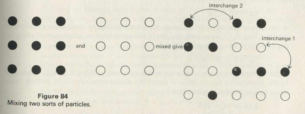
Figure 84: Mixing two sorts of particles.
Full Size Image
The mixture can be arranged in many ways. Exchanges of unlike particles, such as interchange 1, make a difference. Exchanges of like particles, however, such as interchange 2, make no difference.
Now suppose one more black particle is added, there being N particles in all, and that there were previously W ways of interchanging particles which made a difference. The extra particle can be interchanged with all N other particles, multiplying W by N, but N/2 of these interchanges are with particles just like the added one, so these ways must be discounted, and N � W must be divided by N/2. The net effect is to double the number of ways, dividing W by the fraction, 1/2, of particles like the extra particle.
Note to teachers
If there are N particles, n1 of one sort and n2 of another, the number of interchanges is W = N!/n1! n2!. Adding one particle of the first sort increases N to N + 1, and n1 to n1 + 1, multiplying W by (N + 1)/(n1 + 1). When the numbers are large, this multiplying factor is nearly N/n1, or 1/f, where f is the mole fraction of particles of type 1.
In general, if the added particle is like others which are present as a fraction f, less than one, W is multiplied by 1/f when the extra particle is added.
Thus Wafter/Wbefore = Δ ln W = ln 1/f
for one molecule added. For one mole of molecules added, to very many moles already present, the increase is just L times as much, where L is the number of particles in a mole, the Avogadro constant. Multiplying Δ ln W also by k, we obtain, per mole of added constituent,
ΔS = kL ln 1/f.
In the case of the water dissociating, there are two added new kinds of particles, the OH- and H3O+ ions, both present in the same fraction f, both contributing to the entropy in equal amounts, giving
ΔS = 2 kL ln 1/f.
If this increase in entropy is as large as the decrease, - 268 J K-1 mol-1, incurred by the dissociation of one mole of water, the dissociation can occur. Putting them equal to one another, we can find f:
2 kL ln 1/f = 268
ln 1/f = 16
1/f = e16 = 107
f = 10-7
f is better known in this context as the hydrogen ion concentration in pure water, and its negative power of ten as the pH, equal to 7, of pure water.
Notice that in a dilute mixture, where f is a small fraction and 1/f is large, the entropy gain from adding another few particles is very large. It is for this reason that chemical reactions rarely go to completion. However large the entropy penalty for running the reaction backwards, the formation of just a few molecules of a kind different from the majority gives such a large increase in mixture entropy, that a few such particles are always formed.
Note to teachers: equilibrium constant expressions
The general equation for chemical equilibrium can now be written down. It is
ΔSconcentrations + ΔSchemicals + ΔSsurroundings = 0
In the simple reaction of the type A = B, the conversion of one mole of A to B alters the first entropy term by
ΔS = kL{ln 1/[B]-ln 1/[A]} = -kL ln [B]/[A]
where [A] and [B] are the mole fractions, or molar concentrations, of A and B. The quantity [B]/[A] is the equilibrium constant K. For more complex reactions a similar argument again leads to
ΔS = -kL ln K.
Putting these things together, using the subscript σ to denote the chemical system, and writing R = kL, we have
-R ln K + ΔSσ-ΔHσ/T = 0
or ln K = ΔSσ/R-ΔHσ/RT
and ln K = -ΔGσ/RT
writing ΔG = ΔH -TΔS.
Thus we arrive at the usual chemical expression for the equilibrium constant in terms of the Gibbs free energy ΔG.
Example 7: Inefficient engines
The car engine discussed in Part Two was pretty inefficient; about 70 per cent of the fuel energy merely went directly to warm the atmosphere. If such waste could be eliminated, a car could go three times further on a tankful of petrol than it can now.
Power stations are more efficient than cars, but even the best of them pass 60 per cent of the energy obtained from the fuel they use, out through cooling towers, or into rivers. This energy can be used for warming nearby blocks of flats, as is done at Battersea in London, but it is usually wasted and it never goes into the electrical energy supplied by the station.
The efficiencies of power stations vary a good deal. Figure 85 shows the efficiencies of power stations in the south east of England, plotted against the temperature of the steam delivered to their turbines.
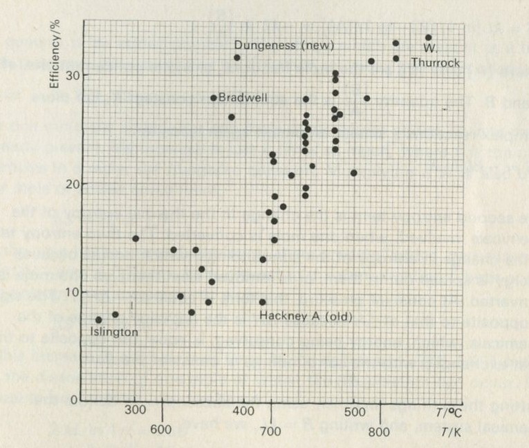
Figure 85: Power stations in CEGB South Eastern Region. Efficiency plotted against steam temperature. Data from CEGB (1968) Statistical yearbook.
Full Size Image
Figure 85 suggests that the efficiency of a power station is related to the steam temperature, because the points lie clustered along an upward-sloping line, from low temperature, low efficiency stations like Islington, to high temperature, high efficiency stations like West Thurrock. It is also clear that factors other than temperature are important. An old power station like Hackney A has a much lower efficiency than a new one like Dungeness, although the temperatures involved are very similar. Clearly, good design, unrelated to steam temperature, counts for a good deal. Nevertheless, the temperature is of the greatest importance, and we shall see why in a moment.
The earliest steam engines, such as the one shown in figure 86, were notably inefficient. One of the main uses of these early engines was in pumping water from mines, though they soon found many other industrial uses, and powered the cotton mills which gave an early impetus to the Industrial Revolution. At first, people had no idea of whether such engines were close to, or far from, the best efficiency that could be hoped for. A young French engineer, Sadi Carnot, was the first to realize that all such engines must be inefficient to some extent. Out of Carnot's ideas there grew the concept of entropy, and the principle that, in any natural process, the entropy will not diminish. Nowadays we can approach the matter the other way round, seeing how an understanding of entropy leads to the fact that an engine extracting energy from a hot body like the boiler of a steam engine, must necessarily be inefficient to some extent.
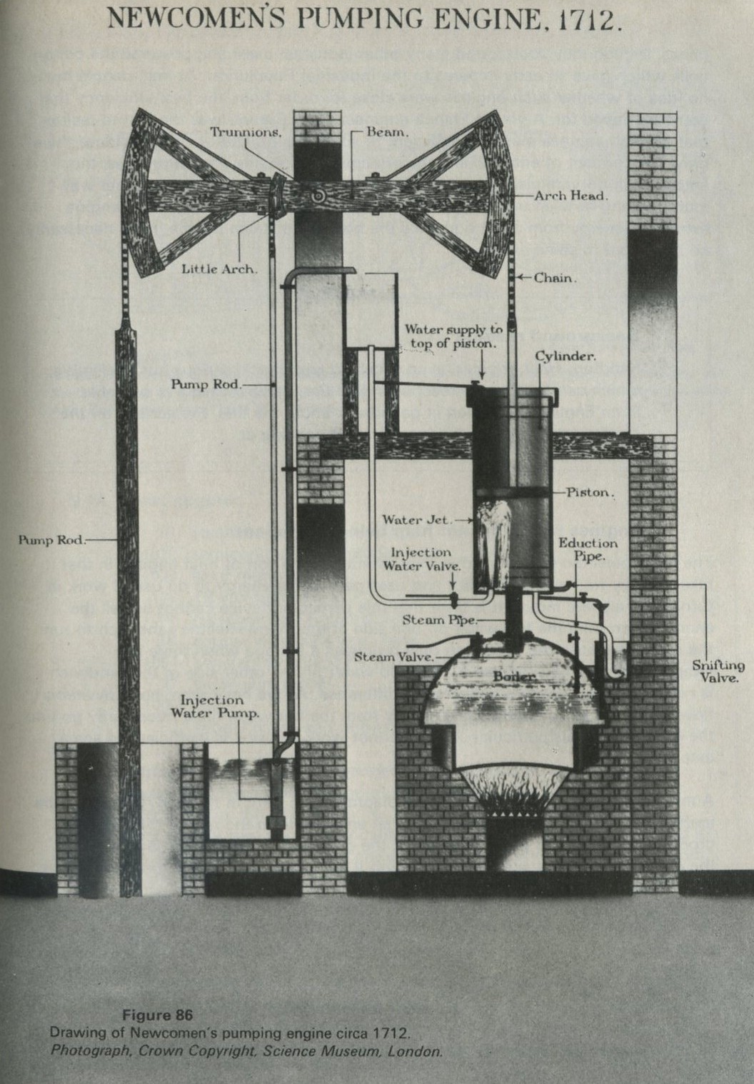
Figure 86: Drawing of Newcomen's pumping engine circa 1712. Photograph Crown Copyright Science Museum London.
Full Size Image
Background reading
Sandfort, Heat engines, is an excellent paperback, serious but intelligible, which can be strongly recommended. Carnot's own work is available in an English translation in paperback under the title, Reflections on the motive power of fire, and is well worth looking at.
Engines which cannot help being inefficient
The thermoelectric device used in experiment 9.6 is a sort of heat engine, in that it takes energy from something hot and uses part of this energy to do useful work in turning an electric motor. It is clear that this particular device cannot use all the energy taken from the hot water on one side of the thermoelectric sandwich to run the motor, because the sandwich only produces a voltage when there is a temperature difference across it. The cold water on the other side of the sandwich is needed to maintain this temperature difference. As we have seen, heat inevitably flows from hot to cold, and some energy from the hot water must necessarily go into the cold water. This particular engine cannot work unless it is inefficient to some extent.
A modern aircraft jet engine, shown in diagrammatic form in figure 87, must also be inefficient if it is to work at all. The gas jet emerges from the rear of the engine, producing a thrust. To produce a thrust, the gas must emerge faster than it enters the engine, and this is achieved by making it hot. Just because the gas is hot, there must be an energy transfer as the gas in the jet stream cools to the temperature of the surroundings, and this energy transfer does not contribute to the kinetic energy of the aircraft.
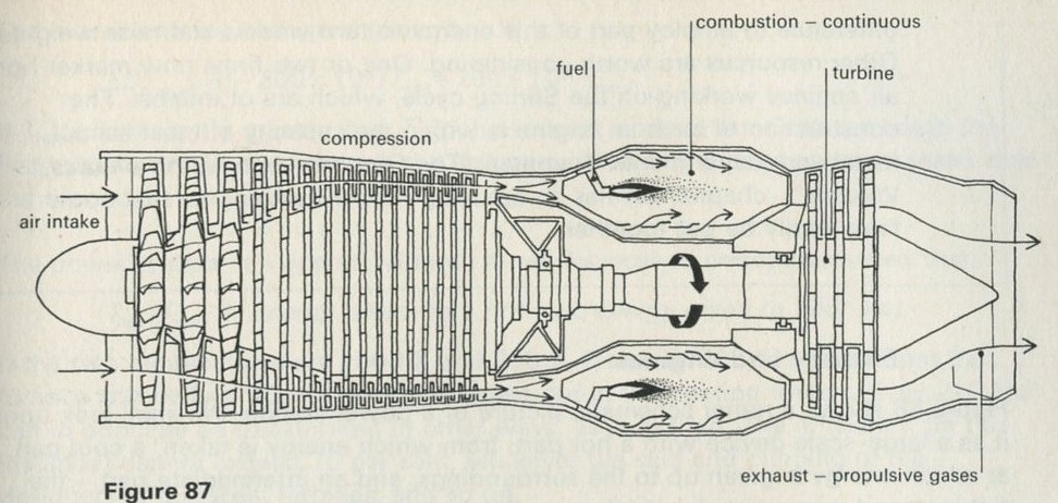
Figure 87: A turbojet aero engine. More recent engines have more than one stage of compression, and also use the compressor to contribute cool, high velocity air to the jet; this air bypasses the combustion stage. After Rolls-Royce Ltd (1966) The jet engine.
Full Size Image
9.14 Heat Engines
    91   steam engine unit
  1072   semiconductor thermopile unit 1023 solar motor
   176   12 volt battery
  1001   galvanometer (internal light beam)
    28   copper wire, 32 s.w.g., bare
  1054   constantan wire, 32 s.w.g., covered
    77   aluminium block
  1000   leads
         supply of ice and of boiling water
It may be worth showing the thermoelectric engine, already used in experiment 9.6, again. The point to establish is that the device needs a temperature difference in order to work, so that some of the energy from the hot part necessarily cannot appear at the motor, but must go to the cold sink. It is helpful to show that the engine will take energy from cold water if the heat sink is even colder, by putting dry ice and alcohol in the latter; also to show that the engine can be put in reverse, being supplied with energy electrically, and raising energy from the cold side to the hot side.
The model steam engine used in the Nuffield O-level Physics course may be worth seeing again, the main point being to illustrate by more than one example the general notion of a heat engine: a device with a hot source and cold sink, using the flow of energy under this temperature difference to employ part of this energy to turn wheels and raise weights. Other resources are worth considering. One or two firms now market hot air engines working on the Stirling cycle, which are of interest. The construction of such an engine is within the capacity of most school metalwork departments. Feynman (The Feynman lectures on physics, Volume 1, chapter 44) has an amusing rubber heat engine that could fairly easily be put together.
Entropy and engines
Figure 88 shows a rather schematic picture of a power station. We shall look upon it as a large-scale device with a hot part, from which energy is taken, a cool part, at which energy is given up to the surroundings, and an intermediate part - the turbines and dynamos - in which part of the energy flowing through the system is diverted and sent off along cables to do work for consumers.
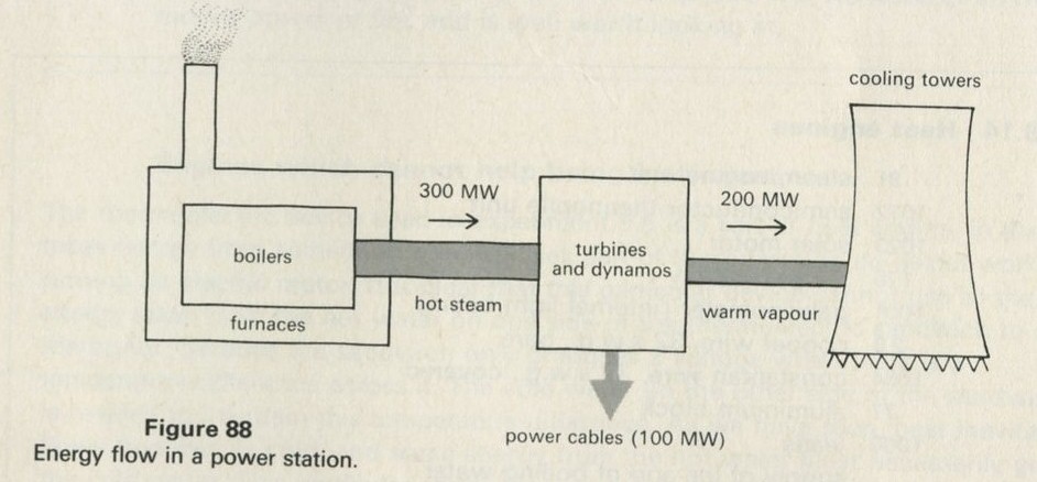
Figure 88: Energy flow in a power station.
Full Size Image
Suppose the station puts out 100 MW of power, and has an efficiency of 33 per cent. 300 MW must be being conveyed from the furnaces to the turbines, 200 MW of which finds its way into the atmosphere via the cooling towers. If the temperature of the hot part is Thot the removal of 300 MJ of energy in one second involves an entropy drop of
ΔShot = -300 � 106/Thot.
But entropy cannot diminish, in any actual process. The compensating entropy increase is to be found at the cooling towers, where the delivery of 200 MJ in one second to the surroundings at the temperature Tcool involves an entropy rise of
ΔScool = + 200 X 106/Tcool
The overall entropy change is given by
ΔSoverall = - 300 � 106/Thot + 200 � 106/Tcool.
If Thot is sufficiently greater than Tcool, the second, positive term can outweigh the first, negative term, even though the first term involves a greater energy transfer than the second.
The power station can operate without a net decrease in entropy provided that
Thot/Tcool > energy taken from hot part/energy given to cool part.
If the two temperatures are 1000 K and 300 K, for every 300 MJ taken from the furnace and boilers, 90 MJ must be passed out at the cooling towers. Only 210 MJ can in principle be transformed in other ways, as is desired. The efficiency (in this instance) cannot exceed 70 per cent, whatever the skill and cunning of the designers of furnaces, turbines, and so on.
The efficiency of modern power stations approaches one half of their maximum possible efficiency, whereas when Carnot made his first calculations, the best attained by steam engines was put by him at about 1/20 of the possible efficiency. There is still plenty of scope, within the restriction imposed by the need for entropy to increase, for skilful design.
It should also be clear that, to obtain high efficiency, the general rule is the hotter the better. That is why in engines of most sorts, and especially in steam engines and turbines, the operating temperatures have been climbing over the years. The earliest steam engines operated with steam at atmospheric pressure, and so at 373 K. If the exhaust were at 300 K, a fraction 300/373, or 80 per cent of the energy taken from the boiler would have had to be wasted, with a maximum attainable efficiency of 20 per cent. In a modern power station, as may be seen from figure 85, the steam enters the turbines at over 800 K. In a modern jet engine, the working temperature is higher still, with the turbine having to run with its blades glowing hot. The use of these high temperatures produces many problems, notably of corrosion and of reduced strength of moving parts, but high temperatures are so desirable on grounds of efficiency that it is well worth while devising new methods and materials so as to permit their use.
Example 8: Cells as energy converting devices
Energy from electron transfer reactions
When zinc dust is put into copper sulphate solution, the mixture becomes warm. Zinc atoms become charged zinc ions Zn2+(aq) in solution, and charged copper ions Cu2+(aq) come out of solution, becoming uncharged copper atoms. The net effect is the transfer of electrons from zinc atoms to copper ions, as the equations which follow indicate:
Zn(s) → Zn2+(aq) + 2e-
2e- + Cu2+(aq) → Cu(s)
The reaction delivers energy (some 217 kJ, when one mole of zinc atoms becomes zinc ions in this reaction). It would be a good thing if the electrons could be made to go from the zinc to the copper along a wire through a motor, rather than for the reaction to take place all in one test-tube, because then the motor might be able to lift a load, which would be a more useful outcome than the mere warming of the contents of the test-tube.
The trick can be achieved by dipping zinc into zinc sulphate, copper into copper sulphate, joining the metals with a wire, and keeping the two solutions apart with a porous barrier. This particular cell is called the Daniell cell, but many others are known. Dry cells, lead-acid accumulators, and the mercury cells used in transistorized deaf aids all use the same basic idea: an electron transfer reaction is made to happen by taking the electrons from one place to another through a wire, and on the journey, energy is transformed.
Entropy effects on a cell voltage
A cell, not unlike the Daniell cell, but in which electrons are transferred from copper atoms to silver ions, is more suitable than the Daniell cell for making observations of the effect of entropy changes on the maximum voltage delivered by the cell, because the entropy change of its constituents is larger than that in the Daniell cell.
The cell is shown in figure 89. A copper wire dips into copper sulphate solution. On the other side of a porous barrier, a silver wire dips into silver nitrate solution, and the two wires form the cell's electrodes. When one mole of copper atoms become copper ions, in the reaction
Cu(s) → Cu2+(aq) + 2e-
two moles of electrons can flow through the wire from copper to silver. Two moles of silver ions can then become silver atoms, being deposited on the silver wire.
2Ag+(aq) + 2e- → 2Ag(s)
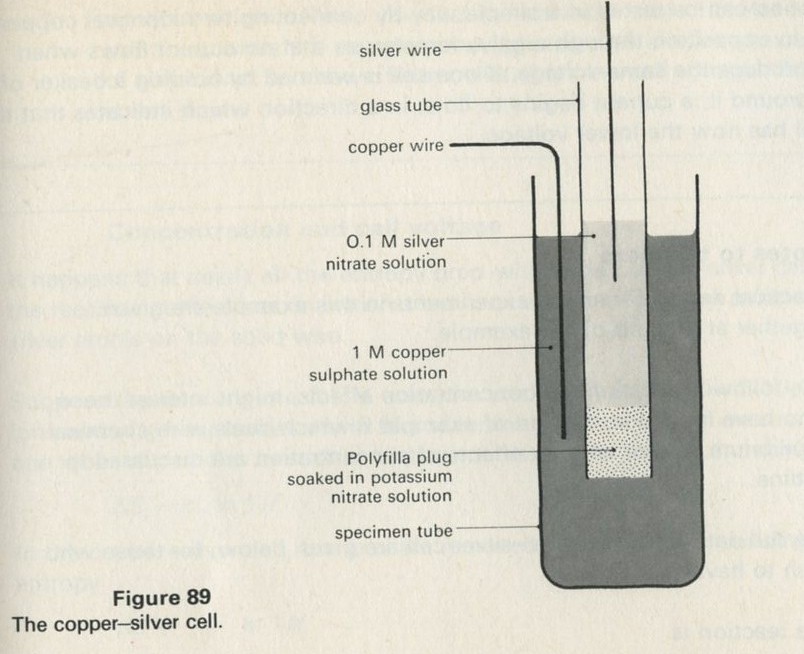
Figure 89: The copper-silver cell.
Full Size Image
The maximum cell voltage is rather less than half a volt. When one mole of copper atoms and two moles of silver ions take part in the electron transfer reaction, the energy liberated is 146.8 kJ. The entropy of the constituents decreases by 193 J K-1 when one mole of copper atoms becomes copper ions in this reaction. Entropy cannot decrease, so to compensate, entropy must increase by at least 193 J K-1 elsewhere. This can be achieved by using part of the energy of the reaction to warm the surroundings. At 298 K, the amount needed is TΔS = 193 � 298 = 57.6 kJ out of the 146.8 kJ available. Thus 146.8- 57.6 = 89.2 kJ are available to be delivered as work by the flow of electrons. Two moles of electrons carry charge 2 � 96 500 C. The maximum cell voltage is thus given by the energy available divided by the charge flowing.
V = 89.2 � 103/96 500 � 2 = 0.46 V.
What will happen if the cell is made warmer? The entropy increase ΔS= 193 J K-1 must still take place in the surroundings. If the surroundings become hotter, the energy needed to produce this entropy increase (given by TΔS) is correspondingly bigger. Less of the reaction energy is available to be transformed electrically. The maximum cell voltage must fall.
This prediction can be tested in a simple way by connecting two identical copper-silver cells in opposition through a galvanometer, so that no current flows when they both produce the same voltage. If one cell is warmed by holding a beaker of hot water around it, a current begins to flow, in a direction which indicates that the warmer cell has now the lower voltage.
Notes to teachers
Practical details for all the experiments in this example are given together at the end of the example.
The following section, on concentration effects, might interest those who have looked at the part of example 6 which deals with chemical equilibrium, where entropy effects of concentration are discussed in outline.
The full data for the copper-silver cell are given below, for those who wish to have them.
The reaction is
2Ag+(aq) + Cu(s) = 2Ag(s) + Cu2+(aq)
At 298 K, for two moles of silver ions and one mole of copper atoms reacting, the thermochemical data are as in table 12.
                 ΔHθ/kJ  ΔSθ/J K-1  TΔSθ/kJ  ΔGθ=ΔHθ-TΔSθ/kJ  Eθ/V (=ΔGθ/2F)
A              -211.2   -191       -57.0      -154.2          +0.80
B               +64.4   -2         -0.6       +65.0           -0.34
net reaction   -146.8   -193       -57.6      -89.2           +0.46

A is 2Ag+ → 2Ag(s)
B is Cu(s) → Cu2+(aq)
Table 12
(Symbols: H, enthalpy U+PV; S, entropy of the chemical part of the system; T, absolute temperature; G, Gibbs free energy H-TS; E, cell e.m.f.; F, Faraday, 96 500 C; θ, standard state.)
Because ΔH is not very temperature-dependent, the value of dE/dT is approximately equal to d(TΔS/2F)/dT, or to ΔS/2F. Using the value above for ΔS gives dE/dT ≈ 1 mV K-1.
The entropy change quoted (193 J K-1) can be obtained from the variation of cell e.m.f., in which case the previous argument is circular. But the entropy change can also be obtained indirectly, by measurements of the heat exchanged when ions go into, or out of, aqueous solution. Note also that the values in table 12 refer to molar solutions, while the experiment suggested uses a lower concentration of silver ions. As shown below, this alters the cell voltage. The effect is not large.
Concentration and cell voltage
It happens that nearly all the entropy drop within the copper-silver cell happens in the reaction at the silver, in which silver ions are removed from solution, to become silver atoms on the solid wire.
Suppose the ions are in a 0.1 M solution, so that a fraction, f = 1/10, of the silver ions and water molecules are in fact silver ions. In example 6, we saw that adding one mole of particles to such a mixture increased the mixing entropy by
ΔS = kL ln 1/f.
In the copper-silver cell, the ions are removed, giving a corresponding drop in entropy
ΔS = -kL ln 1/f.
If 1/f= 10, as in a 0.1 M solution, the entropy change is substantial. If the solution of silver ions is made more dilute, so that 1/f is 100 or 1000, the entropy penalty for removing ions becomes even greater. The net entropy drop for the cell will become even larger than before, and yet more of the available energy will have to go to the surroundings to produce a compensating entropy increase. Less energy will be available to be transformed electrically, and the cell voltage will drop.
This prediction can be tested with the pair of cells connected in opposition which were used previously. If almost all the silver nitrate is poured away, and replaced by distilled water, a dilution of at least 100 times can easily be achieved. The cell voltage at once falls.
Demonstration or experiment: 9.15 Energy from cells
9.15a Energy from an electron transfer reaction
1056 1 M copper sulphate solution, 5 cm3
1056 zinc dust, 0.5 g
1055 test-tube, hard glass, 150 � 25 mm
542 thermometer (-10 to 110�C)
Add 0.5 g of zinc dust to 5 cm3 of 1 M copper sulphate solution in a test-tube. If students do it, they can feel the warmth produced. As a demonstration, the experiment is more effective with an electrical thermometer giving an indication on a demonstration meter, than with a mercury thermometer. The zinc must be in dust form: the granulated variety reacts too slowly.
9.15b Entropy effects in a copper-silver cell
   1055  specimen tube 2
   1055  teat pipette
   1056  1 M copper sulphate solution
   1056  0.1 M silver nitrate solution
   1056  saturated potassium nitrate solution
   1056  silver wire, 50 mm 2
   1054  copper wire, 14 s.w.g., bare
   1054  glass tube, 10 mm bore, 50 mm long
   1053  Polyfilla (see below)
     52  K crocodile clip 2
  512/1  beaker, 250 cm3
   1001  galvanometer (internal light beam)
   1000  leads
         supply of ice, hot water, distilled water

Extra items needed if only one cell is used

   1006   electrometer
 1003/1   milliammeter (1 mA) or other display meter for electrometer
   1041   potentiometer holder
          with
   1051   preset potentiometer, 5 kΩ
   1033   cell holder with U2 cell
The most effective demonstration uses a pair of identical cells, though it is possible to use only one (see below). The cells are prepared as follows. Well before they are needed, porous plugs are made in the ends of the 10 mm diameter glass tubes, by pressing these ends into a firm paste of Polyfilla and water, until a plug 10 mm long is formed in the tube. When the plugs are set, the tubes are left standing in saturated potassium nitrate solution until they are needed, so that the plugs are soaked in this electrolyte.
The cells are then made up as in figures 89 and 90, by filling the glass tubes with 0.1 M silver nitrate solution using a teat pipette, and resting them in specimen tubes containing 1 M copper sulphate solution, into which dip the ends of a copper wire. Short silver wires are then dipped into the silver nitrate in the glass tubes.
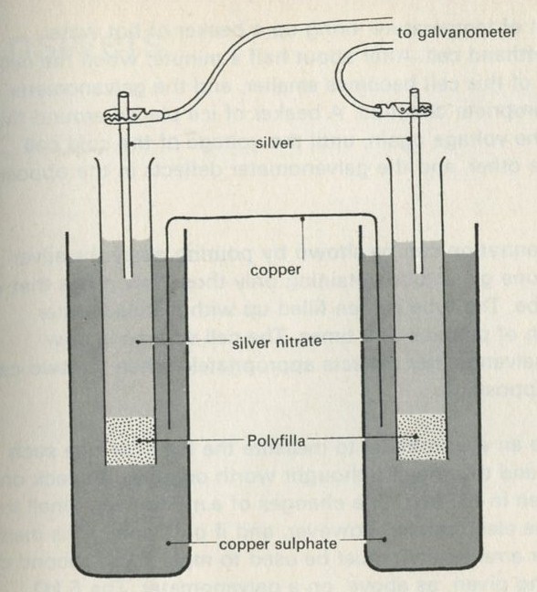
Figure 90: A pair of copper-silver cells in opposition.
Full Size Image
When two such cells are made at the same time, using the same materials and solutions, their e.m.f.s are almost exactly equal, and if the cells are connected in opposition through a galvanometer, the galvanometer gives a negligible deflection. It is convenient, and makes a tidy demonstration, if the two cells are held at their necks by Terry clips fixed to a vertical board. The board can then carry the silver wires soldered to 4 mm sockets ready for connection to the galvanometer. One length of copper wire serves to make the electrodes for both cells, and the connection between them, as in figure 90.
Show first, with the galvanometer connected momentarily across only the lefthand cell (say) with its range at the least sensitive possible, the direction of the deflection from this cell. Then connect the cells in opposition, and increase the sensitivity of the galvanometer, showing that a negligible current flows. It should be possible to use the most sensitive range.
To show the effect of temperature, bring up a beaker of hot water around, say, the lefthand cell. After about half a minute, when the cell is warm, the voltage of this cell becomes smaller, and the galvanometer deflects in the appropriate direction. A beaker of ice placed around this cell will increase the voltage again, until the voltage of the cold cell exceeds that of the other, and the galvanometer deflects in the opposite direction.
The effect of concentration can be shown by pouring away the silver nitrate solution in one glass tube, retaining only those few drops that wet the walls of the tube. The tube is then filled up with distilled water, achieving a dilution of perhaps 100 times. The cell voltage is now reduced, and the galvanometer deflects appropriately when the two cells are connected in opposition.
It is possible to use an electrometer to measure the e.m.f. of one such copper-silver cell, and this may be thought worth doing as a check on the calculation given in the text. The changes of e.m.f. are too small to be shown easily on the electrometer, however, and if only one cell is made up, a potentiometer arrangement must be used to replace the second cell, the indications being given, as above, on a galvanometer. The 5 kΩ preset potentiometer suggested is not easy to use for this purpose, and can with advantage be replaced by a potentiometer with a larger distance of travel between maximum and minimum positions.
Answers
Part 1: One-way processes
1 If the reversed event were a real event, how on earth would the pieces contrive to assemble themselves correctly without help? And how would the necessary energy to lift each piece by the proper amount be gathered together?
2a The sketches were made when the pendulum was at one or other of its maximum displacements, though it is not possible to be sure this is so from inspection of the drawings alone. If you care to guess that it is so, the events are in the proper sequence, because damping is reducing the amplitude of the swings.
2b The sketches are in reverse sequence.
2c It is not possible to tell whether the sequence is in the proper order, or is reversed.
2d This is the correct sequence. The water in the middle can would never, unaided, become hotter at the expense of the water around it, so the drawing containing the larger temperature difference must be the earlier one.
2e In the correct sequence, supposing that the ball is slowing down as it runs from left to right.
3 The energy boxes might look like figure 91.
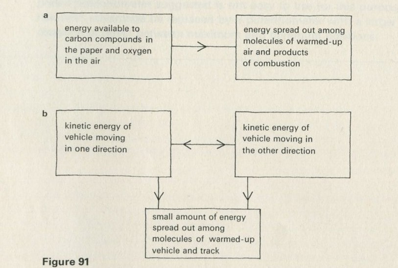
Figure 91
Full Size Image
4Perhaps one might hazard the guess that when a process involves energy being spread out among more objects or among more molecules, its reverse would look absurd. For a good air track, the energy of the vehicle stays almost fixed, and very little leaks away, to become spread out among the molecules of the vehicle and track, making these bodies a shade warmer.
Interestingly, if one started with a number of vehicles at rest on an air track, and sent one vehicle along to collide with them, a film of the resulting motion would also look implausible, even if every vehicle moved without any loss of energy to the track, and all collisions were elastic. Again, a process involving the sharing of energy among many objects is one-way in nature.
5 It is more likely that everyone in a class of three would happen to make the same choice at the same time than that everyone in a class of forty would do so. The chance that any one person will choose to go to the cinema might be the same, but the combined chance that many will do so is smaller than the combined chance that few will do so. If there are, say, six equally favoured ways of spending the evening, one person has six choices. Three students have 6 � 6 � 6 patterns of evening entertainment, while forty have as many as 640 all told.
You would be right to think that the example is artificial. Ways of spending one's time are not equally favoured. If there is a film everyone wants to see, or if there is an organized party, the analysis fails.
6 The Brownian motion looks just as good in reverse as it does in the forward direction. The motion of the jiggling particle (a smokey ash particle in air, for example) is unpredictable in either direction.
7 An electric motor, run in reverse as a dynamo, would be an example.
8 Figure 92 illustrates how a proportion of the energy transformed in the battery goes, via the motor, to lifting a load. That part of the whole process which results in the load being lifted would look plausible in reverse, but to the extent to which the motor becomes warm (current flowing in the resistance of its rotor, for example) the process is one-way.
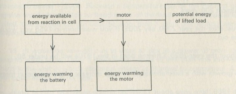
Figure 92
Full Size Image
9 Figure 93 illustrates how all the energy transformed in the battery ultimately goes to warming up the surroundings. The reverse process, with the lamp gathering in energy from around itself, and charging the battery, would be absurd.
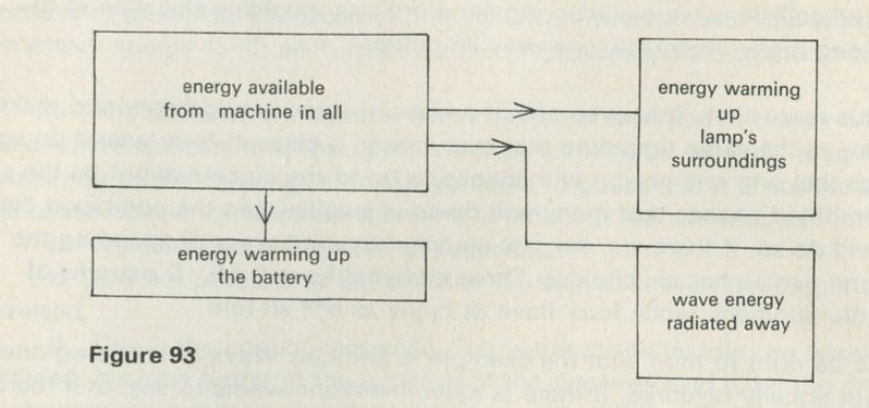
Figure 93
Full Size Image
Note concerning the one-way or two-way nature of a reaction in an electric cell
See Part Six, example 8, for a fuller discussion of the energy-transforming processes in a cell. Whether the cell action warms or cools its surroundings depends on what happens inside the cell. The passage of a current through the cell always delivers energy which goes to warming up the cell and its surroundings, since the cell has a finite resistance, but the cell action may also involve removing some energy from the surroundings. The answer to question 9 is, overall, unaffected, but the answer to question 8 may involve some subtleties.
Part 2: The fuel resources of the Earth
1 Almost 200 years.
2 Just after the year 2000, say 2005. If you were born in 1955 you would be 50 years old.
3 About the year 2020. Children born in the 1970s will be under 50.
4 A growth with a fixed annual percentage increase is exponential in form.
5 In 1969 there were about 11 million private passenger cars in Great Britain. You might have guessed at such a figure by supposing that the population of about 50 million falls into families of rather less than five people each, with rather fewer than one car per family.
6 A car engine can deliver somewhere around 60 or 70 horsepower, say 50 kW. You might reach such a guess by supposing that a car engine is equivalent to a good number of vacuum cleaner electric motors, for example. Or you might know that a car can accelerate to, say, 50 kilometres per hour in a time of the order of 10 seconds, and estimate the power from the rate of increase of kinetic energy, having estimated the mass of a car. Another way would be to reflect that the heater of a car, using perhaps one or two per cent of the engine power, warms the inside of the car not much less quickly than a one kilowatt electric fire would do.
Overall, one might put the power installed in cars at some 500 000 megawatts (5x 10¹¹ W).
7 A power station delivers at least 100 megawatts, often more. You might guess that there are at least 100 power stations in Britain. In 1967-8 there were 216 power stations, with a total capacity of nearly 42 000 megawatts ( 4.2 � 1010 W), an average of just under 200 megawatts each.
Perhaps surprisingly, the power installed in the nation's cars (see question 6) is a whole order of magnitude greater than that installed in its power stations.
8 One way of guessing the total usage of petrol would be to reckon that a car uses some four or five gallons (about 25 litres) of petrol a week, that is, about 20 kg. In a year this amounts to about 1000 kg (1 tonne), so all the cars in the country (see question 5) use about 10 million tonnes. In energy terms, this is between 4 � 1017 and 5 � 1017 J. It represents about 1/25 of all the energy consumed in Britain in a year.
9, 10 The power station is beside a large river. The warming of river water by power stations can have considerable consequences for the animal and vegetable life the rivers can support. Ultimately, the energy used by men warms the Earth until it radiates at a rate sufficient to get rid of the energy delivered to it. At present, the world as a whole is using energy at about 1/10 000 of the rate at which energy arrives from the Sun. But if everyone in the world had the energy standard of living of North America (over five times the world average), the fraction would increase to nearer 1/2000. Because a temperature rise of the Earth of only a few degrees would be enough to flood much of the land area as the polar ice-caps melted, this fraction cannot become more than a small one without serious consequences.
11 It would be very difficult to work all day at a power of more than a hundred watts or so. Thus, a day's work comes to less than one kilowatt hour, which is the unit in which electrical energy is charged to consumers. A kilowatt hour costs about 1p, or less.
12, 13 Less than 1 p (see question 11). The cost of electrical energy is much less than the cost of the food a labourer needs, let alone the cost of wages, so in effect, electrical energy is slave labour. Men as energy-producers alone are far more expensive. In India, for example, this has very direct consequences: it may be cheaper to dig an irrigation canal with machines, but it may be better, in terms of giving people employment, to dig it by manpower.
Part 3: Chance and diffusion
1 No. The marbles could sort themselves out, but unsorted patterns are more likely than sorted ones, because there are more of them.
2 There are very many ways of arranging the marbles so that they are muddled and well mixed.
3 There are fewer arrangements of marbles that one would call well sorted than there are arrangements one would call well mixed. One could argue this from the fact that, given a sorted collection, most changes make it less sorted, but given a mixed arrangement, one has to choose changes with care to move to a better sorted arrangement.
4 Yes.
5 About two times in six.
6 Because there are only two vertically sorted ways as against four not vertically sorted.
7 No.
8 4.88.
9 Yes.
10 One must never expect things to average out too well in the short run.
In the long run, about one picture in sixteen should show the pucks all in one particular half. In thirty-odd frames, it is not too surprising that the pucks never appear together in the lefthand half, nor that they appear three times in the righthand half. In three hundred frames, it would be extremely odd if there were no occasions when all the pucks were in either half.
11 One way would be to toss a coin once for each counter, putting the counter in the righthand or lefthand half according to whether the coin showed heads or tails.
12 No. The average behaviour is with the counters equally spread between the two halves.
13 On the first throw, a counter must move from the full half to the empty half.
14, 15 Five moves out of the six possible moves. The other move will bring the first-moved counter back again.
16 One person in every six.
17 1/W.
18 lg 2100 = 100 lg 2 ≈ 30.
Therefore, 2100 ≈ 1030.
19 1024 seconds.
20 About three million Universe-lifetimes.
Part 4: Thermal equilibrium, temperature, and chance
1 No. The temperatures will have become equal.
2 From the hot water.
3 Because the sandwich is cooler than the hot water.
4 Because it is cooled by the cold can.
5 Not for long. The sandwich would become nearly as hot as the hot can.
6 Because the cold can must keep the sandwich cooler than the temperature of the hot can. Energy going into the cold can is diverted from the motor.
7 No, some goes to the cold can.
8 Energy would seem to come from a dynamo and, going to the sandwich, would seem to appear in one can which became hotter. At the same time some more energy would seem to go from the other can, which would seem to grow cooler. This energy would also seem to be arriving in the can which was growing hotter.
9 That if put in contact, neither will grow hotter or cooler.
10 No, and no again! Your bath water is much more expensive to heat than the hot water in a cup of coffee. But the second may well be the hotter. To bring both lots of water to the same temperature requires quite different amounts of energy. The amount of energy needed to warm something by a certain amount depends on what it is, and on how much of it there is.
11 It will oscillate.
12 Yes. Energy would tend to be transferred from one to the others.
13 It would soon follow the others.
14 Record A would be different; B would be much the same.
15 Always more atoms with n quanta than with n+1.
16 Not the same.
17 The ratios of the numbers of atoms in adjacent energy levels show some very rough tendency to be the same, though the evidence that the ratio is constant could hardly be called convincing.
18 Aspect b. The distribution describes the relative numbers of atoms in the various levels.
19a No.
19b Yes, more or less. Pretty well all games will end up with more atoms in each level than in any higher level. The overall behaviour can be predicted, but not the detailed pattern within that overall behaviour. If you tossed a coin a thousand times, you could predict about how many heads you would get, but not which tosses would give heads.
20 No. It was told to move quanta completely at random.
21 No. The moves were quite random. That is a way of saying they are unpredictable.
22 No. It was told to move quanta completely at random.
23 Neither atoms with many quanta, nor atoms with few quanta, come in for special favour by the random choice of atoms. But if there are many atoms with a certain energy, a lot of random choices will chance to fall on one or other of them.
24a No.
24b Yes, there are so many of them that random choice will tend to hit upon one.
24c Yes, for the same reason.
24d Yes, for the reasons given in a and b combined.
24e Yes. Despite not knowing where to go, the random moves go somewhere definite.
25 Yes.
26 No.
27 Different atoms have each particular possible energy.
28 There is no real change in the numbers of atoms with each particular energy. The distribution is much the same.
29 It ends up with the same number of atoms having each particular energy.
30 It fluctuated up and down around the steady general shape, which did not alter.
31 It would go back to a distribution such as the one shown in figure 40.
This is a puzzling problem. If a series of random numbers choosing sites are random one way, are they not random in reverse order? Yes, if the reversed order numbers were used starting at figure 39, the effect would be to produce the distribution of figure 40, as in all other instances in these films. But applied to figure 40, with the quanta just as they are placed in that figure (not just with the same distribution) this is the one set of random choices that leads back to figure 39, where random choices ought not to go! How was that set found? By picking out the one and only random set of choices that will lead there. But millions of other sets of random choices would lead to figure 41, so the chance of hitting upon just this one set by accident, rather than choosing it with hindsight, is negligibly small (though not zero).
32a Very nearly 2.0.
32b Very nearly 2.0.
32c Very nearly 2.0.
32d The ratios of numbers of atoms in adjacent energy levels is constant, and equal to 2.0.
32e The ratio of numbers of atoms decaying in successive equal time intervals is constant. The decay has an exponential form.
32f Exponential.
33a Yes, pretty well constant.
33b No. The ratio is close to 4.0.
33c See table 13.
Figure No.   N      q    N/q   1+N/q     Distribution ratio
   42       900    900   1.0   2.0           ≈ 2.0
   60       900    300   3.0   4.0           ≈ 4.0
   65      1800   1200   1.5   2.5           ≈ 2.5 (both)
   50       625    625   1.0   2.0           ≈ 2.0
Table 13: Comparison of predictions of distribution ratios with results from the computer simulation on film.
34 In figure 50 there are fewer atoms in all than in figure 42, and there are fewer atoms in each energy level. But in both there are twice as many atoms in each level as in the adjacent higher level.
They are the same in this sense: they have the same proportion of atoms to quanta.
35a No. It was told to move quanta at random.
35b No. They came about quite by chance. Another time the energies could be different.
35c Yes. It happens every time we try.
36a From the less sloping, or shallower distribution, to the more steeply sloping distribution.
36b From high temperature to low.
36c Their general shape no longer changes, apart from fluctuations around that shape. The two distributions continue to have the same shape, and the same steepness, as each other.
36d When the casserole's temperature is equal to that of the oven walls.
36e The lefthand half was hotter than the righthand half in figure 63. In figure 64, the two halves are equally hot.
36f Large ratios of numbers of atoms in adjacent energy levels go with low temperatures, and vice versa.
37a There is a steady small chance that one will get a cold. Because the school has some hundreds of students, there is usually just about the expected proportion of students absent.
37b No - at least we didn't tell it!
37c Very fair. In fact it sums it up nicely.
Appendices
A: Heat, work, the conservation of energy, and the First Law of Thermodynamics
This Appendix was written mainly to clear our own minds. It may be of use to teachers who wish to have a summary of some of these ideas, and of the difficulties involved in them. Most of the ideas will appear only in treatments of thermodynamics that go beyond the requirements of a sixth form course. The ideas outlined below are subtle, hard to grasp, and need play no part in teaching at sixth form level other than in indicating potential confusions to be avoided.
At the microscopic or atomic level, if the conservation of energy holds good, the sum total of the energies of any collection of atoms remains constant, however this energy may be redistributed among them. Of course, all atoms taking part in the energy transactions must be counted in.
At the macroscopic level, for matter in bulk, a parallel - but not identical - principle can be found; the First Law of Thermodynamics. Such difference as there is between the First Law and the energy conservation principle turns on the possibility of making up a macroscopic thermodynamics which does not depend on a microscopic interpretation. Macroscopic thermodynamics depends only on the results of macroscopic experiments. Reasons can be given on a microscopic picture why these macroscopic experiments turn out as they do. The reasons are not necessary to the development of macroscopic thermodynamics, but they illuminate it. Such reasons appear below.
One central concept of macroscopic thermodynamics is that of the parameter of a system. On a microscopic view, a system is a collection of very many atoms interacting with each other. If there are only a few atoms, there is little more to say. But if there are very many, say 1023, a new simplicity emerges. The behaviour of a collection of many atoms will have very stable average properties. In a gas, for example, the number and the velocity of atoms hitting a wall will both have steady average values. At the macroscopic level, as a result, a steady pressure exists, and can be picked out as one of the parameters of this system.
Macroscopically, the existence of a measurable, stable parameter pressure is just a fact of experiment, and might still be true were the microscopic gloss quite wrong (if, say, matter were continuous rather than atomic). Similar remarks can be made about other macroscopic thermodynamic ideas, but we shall not labour the point. Note, however, that if the atomic gloss is right, macroscopic thermodynamics only works for large enough lumps of matter. Two or three molecules in a box have nothing that can decently be called a pressure.
Similar remarks apply to the state of a macroscopic system. Microscopically, the large numbers of atoms involved ensure that the average overall behaviour of the collection will stay much the same, despite an enormous variety of motions and energy interchanges among the atoms. Two boxes of the same gas, both with 1023 molecules and the same total energy will inevitably behave in a quite similar way, even though their detailed atomic motions are utterly dissimilar. The powerful effects of statistical averaging ensure that a large enough system will have a definite state fixed by only a few parameters (pressure, temperature, and density, for example, each of which is a statistical average). Again, a collection of only a few molecules has no such state in the thermodynamic sense, for the actual individual motions of the molecules are very important in deciding its future behaviour, and no simple stable average behaviour emerges.
The above remarks serve to introduce the distinction between the conservation of the energy of a collection of many molecules, and the First Law of Thermodynamics applied to such a system. Conservation of energy says that there will exist a fixed total energy. The First Law says that there exists a quantity U, the internal energy, that will be the same for a system whenever its (few) thermodynamic parameters are the same.
For a gas sealed off in a rigid, insulated box, conservation of energy ensures that there will be a fixed total energy. But the First Law adds that the internal energy will have the same value whenever the gas has the same pressure, temperature, and density, that is, when it is in the same state.
Briefly, the internal energy U is a function of state. For only a few molecules, this makes no sense, though energy conservation still holds. There now exists no simple average behaviour and the total energy, though it has a definite value, cannot be simply related to a few parameters that describe any such collection as a whole, for every such small collection behaves quite differently from every other one. Crudely, the First Law equals energy conservation plus the existence of the statistical equilibrium behaviour of large numbers of atoms. Energy conservation is obeyed, so far as we know, by all-collections of atoms. The First Law is only obeyed, and at that only on average, by collections of very many atoms.
Work, the product of force and distance, can best be regarded as a means of energy transfer. On a classical, non-quantum, atomic picture, work is essentially the only means of energy transfer between atoms. The classical atoms exert forces on one another and exchange energy smoothly as they move relative to one another. On a quantum picture, energy changes are not smooth and work is not such a useful concept. On this picture, the atoms of a system have access to a number of energy levels, and all changes involve either the passage of atoms from one level to another. or the alteration of the energies of the levels, or both. Transitions between the energy levels become the primitive concept that replaces the idea of work.
At the macroscopic level, work is, as usual, the product of a force and distance, or, in general, of a pair of quantities analogous to these two. But here the forces are statistical average quantities over many atoms. If the number of atoms were small, the macroscopic work would have to be replaced classically by a sum of force-multiplied-by-distance calculations for individual atoms or, on a quantum picture, by a sum over changes in the quantized energy levels of a collection of atoms.
Heat, unlike work, is a wholly macroscopic concept. There is no meaning whatever to be attached to the heat exchanged by a pair of atoms. We may interpret heat as the transfer of energy between collections of large numbers of atoms as they spontaneously reach a statistical equilibrium distribution of energy. This attainment of statistical equilibrium is observed on the large scale as the attainment of thermal equilibrium by a system which initially has temperature differences between parts of itself. Thus heat flow only occurs from hot bodies to cold ones. An energy transfer not of this sort is not heat flow.
This use of the word heat is in part at odds with its everyday use. We usually speak of the heat stored in a storage heater, for instance. A thermodynamicist would regard the storage heater as having been given extra internal energy, and would point out that the internal energy had been raised by working electrically, not by heating the radiator. He would agree with the rest of us, however, that there is a flow of heat from the radiator to the room it is intended to warm, for this energy flow comes about as the system room-plus-heater moves towards thermal equilibrium.
Macroscopically, heat can be given meaning independently of any microscopic interpretation. The variation of the internal energy of a system with its pressure, density, and other parameters, can be mapped out by adding or removing energy by way of work alone. Finding that other changes can occur, such as those in which a gas cools without contracting, in which the internal energy change is no longer equal to the work, the heat flow is defined as the difference between them. But this viewpoint, being purely macroscopic, conceals the feature that heat flow, unlike total energy, is a concept with only a macroscopic meaning.
In short, heat flow occurs when systems move towards thermal equilibrium, and thermal equilibrium is a wholly statistical phenomenon, of systems containing large numbers of atoms. It has no counterpart in collections of only a few atoms.
Except in the usage of ordinary language, and by implication in the usage heat capacity, heat is not the same as the energy content of a body. Nor is it an identifiable part of this energy content. The internal energy of a body may change by way of work, or by way of heat flow, or by way of both. Heat is a bird of passage; a way of changing the internal energy of things, not a quantity they can contain.
We repeat that this subtle usage is presented here for information. There is no merit in pressing it upon students before they can understand that there is a case for modifying the ordinary usage. Nor is the thermodynamic usage correct and the ordinary one wrong. The thermodynamic usage is convenient and consistent for certain purposes for which the ordinary usage is not.
It may be advisable not to refer to processes such as the warming up of a body by the flow of electricity or by friction as cases of work being turned into heat. In such cases, energy is exchanged by way of work and the internal energy of the body rises and it becomes warmer. The energy has been spread out (or shared out) amongst many atoms or molecules, and it is this which makes the process irreversible. So one may say that the energy, once stored in a battery, or in a moving mass, or in some form of potential energy, has been spread among a large number of atoms.
While it may be good to encourage students to speak in such a manner, it would be premature to insist that they do so.
B: The Einstein model and the Kelvin temperature
The Einstein model makes the approximation that a monatomic solid can be represented by a collection of harmonic oscillators, sufficiently independent of one another for the energy levels of each oscillator to be identical with those of an isolated oscillator, but weakly coupled so that the oscillators share energy with one another.
The energy levels of an isolated oscillator are equally spaced, at intervals ε = hf, where f is the classical oscillation frequency, and h is the Planck constant. The lowest level has the zero point energy �hf, but as the oscillator cannot have less than this energy, the energy of the lowest level can be treated as if it were zero. If all oscillators are alike, they thus exchange energy only in lumps or quanta of energy ε.
The number of ways of arranging quanta of energy on the oscillators may therefore be counted, as in figures 69 and 70, by counting the number of ways of placing marks differently in boxes.
The calculation of W for an Einstein solid
Figure 94 shows a general way of noting down any one arrangement of q quanta amongst N oscillators. The circles stand for oscillators, listed in some definite order. The symbols ε stand for quanta. The energy of each oscillator is indicated by the number of ε symbols which follow it. Thus the first listed oscillator has one quantum, the second has three, the third has none, and so on. The listing carries on until all N oscillators have had their energy specified, so that N symbols o and q symbols ε have been used up.
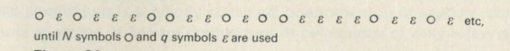
Figure 94: Representation of the state of an Einstein solid.
Full Size Image
Any list of this form, containing N oscillator symbols and q quantum symbols, will represent a possible arrangement of the quanta among the oscillators. W is the number of such lists which are different from each other.
If one has to select a list from n distinct objects, the first choice can be made in n ways, picking any one of the objects. That leaves (n-1) ways to make the second choice, one object having been selected already. Every one of the n first choices can go with every one of the (n-1) second choices, so that the first two choices can be made in n (n-1) ways. The number of ways of making all the choices is given by
n (n-1)(n-2)(n-3) ... (3)(2)(1)
which, for short, is written n! and called factorial n.
In the list of figure 94, the first place must be an oscillator symbol o. That leaves (N+q-1) symbols to play with, and the number of their rearrangements is (N+ q-1)!. But all the q quantum symbols are alike, and interchanging the symbols makes no difference to the listed arrangement (the first atom in figure 94 has one quantum whichever ε symbol is put after it, as long as only one of them is put there). There are q! ways of making these trivial rearrangements of the q quantum symbols. Similarly, after the first oscillator symbol, the remaining (N-1) oscillator symbols can be rearranged among themselves in (N-1)! ways, without making the least difference to the meaning of the list, because the particular oscillators are indicated by their place in the list sequence, not by each having an individual symbol.
Thus W, the total number of distinct rearrangements, is less than (N+q-1)! . Every one of the uninteresting, non-significant rearrangements of oscillator and quantum symbols amongst themselves can go with every rearrangement of any kind. So the number (N+q-1)! must be divided by q! and by (N-1)!. W is then given by
W = (N+q-1)! / (q!(N-1)!)
If N = 3 and q = 3, W becomes
W = 5!/(3!2!) = (5 � 4 � 3 � 2 � 1) / ( (3 � 2 � 1) (2 � 1) ) = 10
Figure 70 shows these 10 ways enumerated one by one.
If the number of quanta is increased by one, to (q+1), the term on the top in the expression for W becomes (N+q)!, which is just (N+q) times larger than it was before, since the factorial is the same list of multiplying terms with an extra term (N + q) in front.
The term q! in the lower line becomes (q+1)!, which is (q+1) times larger than before. The term (N-1)! is unaltered. Thus W is multiplied by the factor (N+q)/(q+1), if one quantum is added. Writing W* for the new number of ways,
W*/W = (N+q)/(q+1) ≈ (1+N/q) if q is much larger than one.
The internal energy and heat capacity of an Einstein solid
Introducing the expression which defines the temperature T,
kT = ε/Δ ln W,
we have, for one quantum added,
kT = ε/ln(1 +N/q)
or
1 +N/q = eε/kT.
If the total internal energy is U, comprising q quanta of energy ε, we can write U/ε in place of q. Doing so, and rearranging the equation, give,
U = 3εL/(eε/kT-1)
where 3L has been written for N, so that the internal energy is given for one mole of atoms, equivalent to 3L independent oscillators.
Putting ε = hf gives the usual expression for the internal energy of one mole of Einstein solid.
The molar heat capacity can be found by calculating dU/dT, giving the prediction, first made by Einstein, that the heat capacity should fall towards zero as T goes towards zero.
Average distribution and most probable distribution
The expression
W*/W =(1 +N/q)
obtained above, for one quantum added to the system, leads, by the argument given in Part Five of the text, to an average distribution of atoms among energy levels which is exponential, the ratio between numbers of atoms in levels of adjacent energy being (1+N/q).
It is also possible to show that this is the most probable distribution. Figure 95 is intended to represent N oscillators placed with n0 having the least possible energy; n1 having one quantum, and so on.
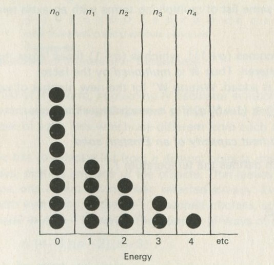
Figure 95
Full Size Image
The N oscillators can be permuted among the energy levels in N! ways. But these ways ignore the fact that the n0! permutations of oscillators in the lowest level, the n1! permutations of those in the first level, and so on, are of no account, since the order in which the oscillators are listed is of no importance. Thus
w = N!/n0n1n2...
gives the number of distinct arrangements for the one distribution in which the level populations are n0, n1, n2 ...
The most popular of such distributions will be the one for which w is largest. w will be at a maximum when a small change in the distribution produces no change in w, using the general property of turning points.
A suitable change which conserves energy in the system is to demote one atom from the j-th level to the one below, the i-th level, and promote one atom to the level above the j-th, the k-th level. Thus
ni → ni + 1
nj → nj - 2
nk → nk + 1
Substituting these new values in the expression for w, we find that w is altered by the factor
ni(ni-1)/(ni+1)(nk+1) ≈ nj 2/nink (1 ≪ n)
The factor will be unity, and w will thus be unchanged and so at its maximum, when
ni/nj = nj/nk,
w is a maximum, belonging to the most probable distribution, when the populations of adjacent levels are in constant ratio, and the distribution is exponential.
This calculation, to be found in many books, often in a more difficult form, has only modest value. It can be extended to give the value of w for the most probable distribution, but this is not the same quantity as W, the total number of distinct states consistent with a given energy. It is W which is needed if one is to make calculations of the behaviour of two systems put together, and it is W which is required for the simplest statement or the basic principle of statistical mechanics, which is that the average behaviour of a large system can be found by averaging over all of the number W of its possible distinct quantum states, giving equal weight to each. (Note that because there may be more than one quantum state with the same energy, it is better to say quantum states here than energy levels.)
The distinction between W and w can be illustrated further by the example of balls partitioned between two halves of a box. The total number of rearrangements W is just 2N, if there are N balls.
If the balls are distributed with n1 in one half and n2 in the other half, this particular distribution can be realized in w = N!/n1! n2! ways. The most popular distribution is that for which n1 = n2.
The maximum value of w, wmax, is always less than the value of W, and the ratio W/wmax becomes larger, not smaller, as N increases. However, ln wmax becomes a better and better approximation to ln W as N increases, and it is this which justifies the substitution of ln wmax for ln W in many treatments of statistical mechanics, despite the lack of fundamental significance of the quantity wmax.
Temperature and level spacing
In Parts Four and Five, the Kelvin temperature of an Einstein solid was defined by means of the equation
kT = ε/ln(1+N/q).
In the only instance of heat flow considered (in the sixth film of the series of computer films, illustrated in figures 61 to 65), the energy level spacings ε in the hot and cold bodies were identical, so that the problem reduced to something analogous to the diffusion of quanta. In this example, the energy level spacing ε plays no part in the argument, and would seem not to be needed in the above expression for the temperature.
The need to include the energy level spacing can be brought out by considering a slightly more complicated example.
Consider an Einstein solid having N oscillators and q = N quanta. The ratio (1+N/q) is equal to 2. A second such solid could have the same mean energy per oscillator, but could have levels of twice the spacing. It would have q=N/2 doubled sized quanta, and the ratio (1+N/q) would be 3.
Now suppose that this second solid gave up one of its (large) quanta. W for this solid would be divided by the factor 3. But if this energy goes to the other solid, it becomes two (small) quanta. Each of these two quanta, when added to the solid containing q = N other (small) quanta, multiplies W for that solid by 2. When both are added, W is multiplied by 2 � 2 = 4.
The effect on W for the pair of solids together, which is the product of W for each alone, is to multiply it by 4/3. Thus the transfer of energy from the solid with fewer, larger quanta to the one with more, smaller quanta, leads to an increase in W overall, and will happen. The solid with the larger quanta was the hotter of the two. It is worth noting in passing that the two solids are not at the same temperature, despite the fact that they have the same mean energy per atom.
In general, we consider a pair of Einstein solids having N, and N2 oscillators; level spacings , and ε2; and numbers of quanta q1 and q2. A small energy transfer dU will represent dU/ε1, quanta added to or removed from solid 1, and dU/ε2 quanta added to or removed from solid 2. The addition of dU/ε quanta multiplies W for either solid by the factor (1 +N/q)dU/ε.
The two will be in equilibrium when these factors are equal; that is, when (taking logarithms)
ε1/ln(1+N1/q1) = ε2/ln(1+N2/q2)
The general expression for this equality reads as
ε1/Δ ln W1 = ε2/Δ ln W2
Because the quantity ε/Δ ln W is what is the same in two systems in thermal equilibrium, it is the quantity chosen for defining the temperature T using
kT = ε/Δ ln W.
Temperature and statistics
The statistical definition of the Kelvin temperature given above is fundamental and comprehensive. Any physical system for which it is possible to measure a quantity related to Δ ln W, when energy is added or removed, can be used to measure Kelvin temperatures. In principle, one could take any material and simply count the number of atoms in two quantum states different by energy ε. If this ratio were, say, 2, and the level spacing ε were 10-20 J, the temperature would be given by
T = 10-20 / k ln 2 ≈ 1 000 K.
Something very close to this is done in practice, when temperatures are measured using paramagnetic salts. For some such salts, an adequate model is to suppose that each atom has a magnetic moment μ, and that each can have its moment either parallel or anti-parallel to an applied flux density B. A moment with its direction anti-parallel to B has extra energy μB; a moment parallel to B has reduced energy -μB. The first requires energy to be taken from the remainder of atoms, leading to fewer ways, and so will be rare. The second gives energy to be shared out, leading to more ways, and so will be common. There are thus more moments parallel to the field than there are moments anti-parallel to it, and the material has a net magnetization along the field. The magnetization varies as
eμB/kT-e-μB/kT
(If kT ≫ μB - weak moments, small field, high temperature - this reduces to
(1 + μB/kT)- (1 - μB/kT) = 2μB/kT
since ex ≈ 1 + x if x is small. This last result is Curie's law: the magnetization varies as 1/T.)
A paramagnetic salt can thus be used as a thermometer, employing the net magnetization of the specimen as a means of counting proportions of atoms in two energy states.
Needless to say, an ideal gas can also be used as a means of measuring Kelvin temperatures. For example, if a gas of N particles increases its volume from V to (V+dV), a statistical argument, like that which gives the factor 2N for the increase in W when the volume doubles, says that W is multiplied by the factor [(V+dV)/V]N. that is,
d(ln W) = N ln(V+dV)/V ≈ N dV/V.
If the expansion is reversible, W does not change overall. If the expansion is also isothermal, the compensating decrease in W comes from heat Q extracted from a heat sink at temperature T, reducing W for the heat sink by an amount given by
d ln W = -Q/kT.
In treatments of thermodynamics based on ideal gas cycles, the equality of the ratios Q/T for fractionally similar, isothermal reversible changes, is offered as a way of defining T. Here we see it as a special case of counting changes of numbers of ways.
Furthermore, the pressure P of the gas can be calculated. In the isothermal, reversible change considered,
P dV+Q = 0
so that P dV= kTd ln W = NkT dV/V
where d ln W is the change either of the heat sink or of the gas. This yields
PV= NkT
which is the usual expression for the pressure of an ideal gas, here obtained from statistical considerations. We now also see why it is common to regard the Boltzmann constant k as the gas constant divided by the number of molecules, and why temperature on the ideal gas scale can be identified with the fundamental statistical Kelvin temperature.
Sources of reference for teachers
Versions of the argument for the most probable distribution appear in
- Bent, The Second law
- Sherwin, Basic concepts of physics
- Millen (ed.), Chemical energetics and the curriculum
- Gurney, Introduction to statistical mechanics
- Sources of physics teaching. Part 1
The argument for the value of W for the Einstein solid is to be found in Bent's, The Second law, Chapters 21 and 22 (which also contains a discussion of the internal energy of an Einstein solid).
The canonical ensemble is discussed in detail in a thorough but tough treatment in Reif, Statistical physics (The Berkeley Physics Course, Volume 5).
C: The quantum shuffling game for indistinguishable quanta
One of the innovations in the text is the introduction of a game in which quanta are shuffled at random between oscillators, the quanta being counters, and the oscillators being sites located in a definite pattern. The six sequences in the film Change and chance; a model of thermal equilibrium in a solid are based on this game. The purpose of this Appendix is to outline the relationship between the game and the more orthodox statistical calculations to be found in books on statistical mechanics.
The rules of the game have been chosen so that the game reaches a statistical equilibrium which is identical with the statistical equilibrium attained by indistinguishable quanta disposed at random amongst oscillators located at distinguishable sites. It is not clear at first sight how any game played with counters which are in fact distinguishable can represent the behaviour of quanta which are not.
The rules are as follows. Each site is assigned a reference number, and sites are chosen at random, using random numbers generated in such a way that no site is favoured over any other. One move of the game consists of two steps. First a site is chosen at random, and one quantum is removed from it, if it has more than zero quanta at that time. Secondly, another site is chosen at random, and the quantum just removed is placed on it.
If the site chosen has no quanta, no quantum can be picked up, and the move is reckoned to be completed. It turns out that it is very important that all such null moves be counted in in the average behaviour of the system, if the game is to reach the required equilibrium. Before discussing this matter, we shall draw attention to the difference between our game and one other, which gives the wrong result.
Another game would simply be to place q counters down at random on N sites. This could be done by choosing the sites one by one, at random, or even by sprinkling the counters from a great height. The outcome would be the binomial distribution, whose shape is suggested in figure 96.
This distribution has a maximum, which for very many counters lies at the mean, with q/N counters per site. Clearly, if there are many more counters than sites, a negligible number of sites will have no counters.
For indistinguishable quanta shared among distinguishable sites, and also for the game whose rules are explained above, the outcome is very different. As indicated in figure 97, the distribution is exponential, so that however large the number of quanta or counters, more sites have no quanta than have any other number, and the numbers of sites with numbers of quanta different by 1 bear a constant ratio to one another.
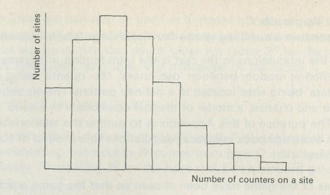
Figure 96: Binomial distribution
Full Size Image
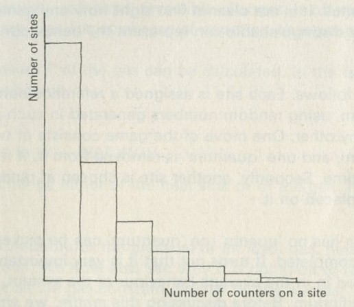
Figure 97: Exponential distribution
The difference arises in quite a simple manner. Consider a three-site system, with two counters. When both counters are on one site, there is no difference between the case where the counters are distinguishable, and the case where they are not, as indicated in figure 98.
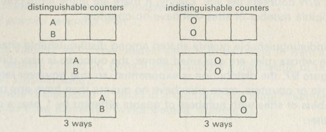
Figure 98
Full Size Image
But when the counters are spread out, with only one site having no counter, there is a difference between the two cases, as illustrated in figure 99. Because interchanging the counters between sites makes a difference when the counters are distinguishable, but makes no difference when they are not, there are twice as many ways of arranging the distinguishable counters as there are of arranging the indistinguishable counters.
The net effect is that, on average, a system with distinguishable counters spends more time in distributions in which few sites have no counters than does a system containing indistinguishable counters. This is the source of the apparently puzzling way in which the indistinguishable counters favour distributions in which many sites have no counters, and sites with few counters are always more frequent than-sites with many counters.
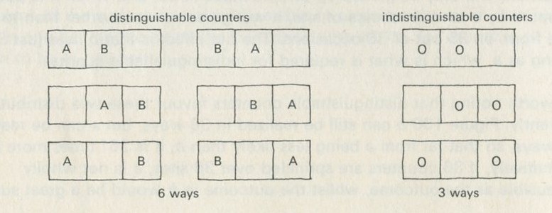
Figure 99
Full Size Image
We now consider, with the aid of a special case, how a game following the rules described can imitate the behaviour of indistinguishable quanta. Figure 100 compares two possibilities for the disposition of 36 counters on 36 sites.
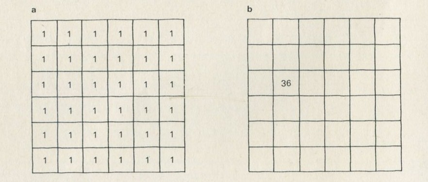
Figure 100
Full Size Image
For indistinguishable quanta, figure 100 a shows a distribution which has just one way of being realized, since no interchanges of quanta make a difference. There is no less likely distribution. Figure 100b shows a distribution that can be realized in 36 ways, depending on which site has the pile of quanta. Thus the distribution shown in b is 36 times more likely than that shown in a.
The game achieves this outcome as follows. The distribution in a will vanish on the next move in 35 out of 36 cases, since only on one move out of 36 will the quantum picked up in the first half of the move happen to be put back on the site it came from, in the second part of the move.
On the other hand, the distribution in b will live much longer, provided that all the moves which hit on an empty site in an attempt to pick up a quantum are counted. A quantum will only be picked up on one move in 36, and when it is put back on the board by a random choice of site, it will go somewhere other than to the site it came from, on 35 out of 36 occasions. The net effect is that b lives just 36 times as long as a, which is what is required for indistinguishable quanta.
It is worth noting that distinguishable counters favour these two distributions quite differently. Figure 100 b can still be realized in 36 ways, but a can be realized in 36! ways, so that far from a being less likely than b, it is 35! times more likely than b. Intuitively, if 36 counters are sprinkled over 36 sites, a is not wholly implausible as the outcome, whilst the outcome in b would be a great surprise.
A full analysis shows that the rules of the quantum shuffling game achieve the proper weight on each possible distribution so as to simulate the distributions of indistinguishable quanta. Such an analysis is given in Black, P. J., Davies, P., and Ogborn, J. M. (1971) A quantum shuffling game for teaching statistical mechanics, American journal of physics, 39, 10, 1154-1159.
D: Photographs of pucks distributed between two halves of a surface
This Appendix consists of two sets of photographs, referred to in the text of Game 9.3 Simulation of the behaviour of marbles in a tray.
The first set, figure 101 a, consists of snapshots of the positions of ten pucks moving about at random on a low friction surface. A white line divides the surface into two equal areas.
The second set, figure 101 b, was made in the same way, but the number of pucks was reduced to four.
Both sets contain enough examples of the distribution of the pucks between the two halves of the surface to make it possible to calculate the mean number of pucks in one half and to study the frequency with which, for example, all the pucks happen to be in one half.
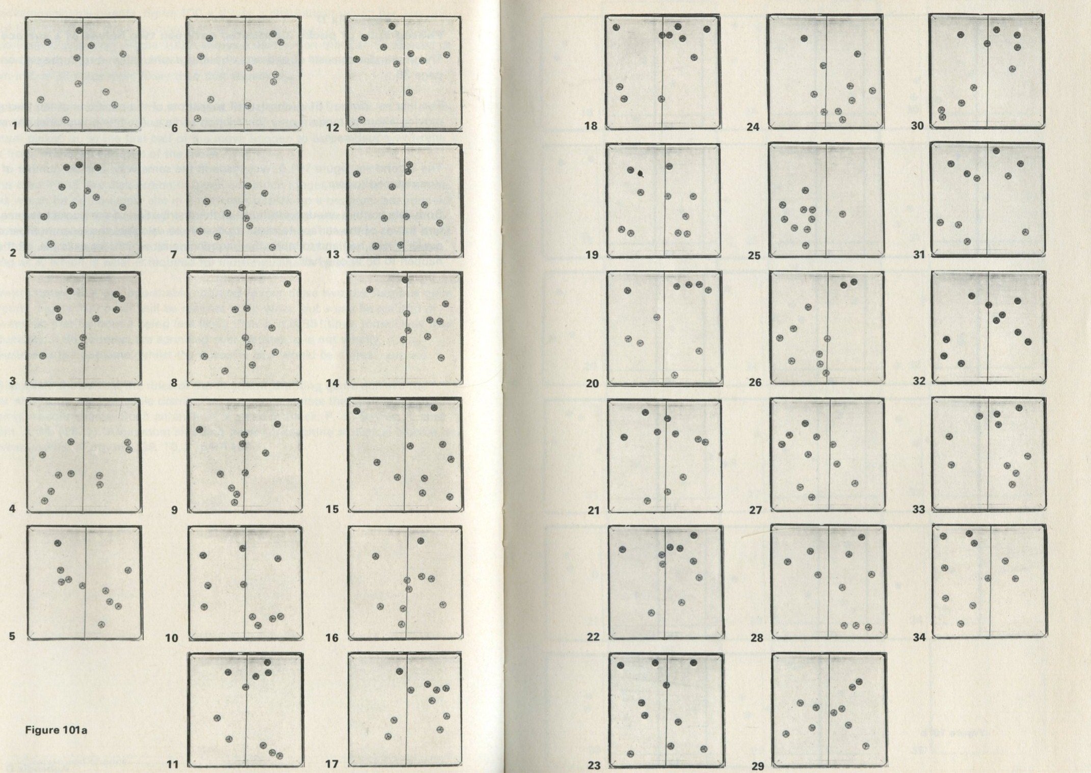
Figure 101a
Full Size Image
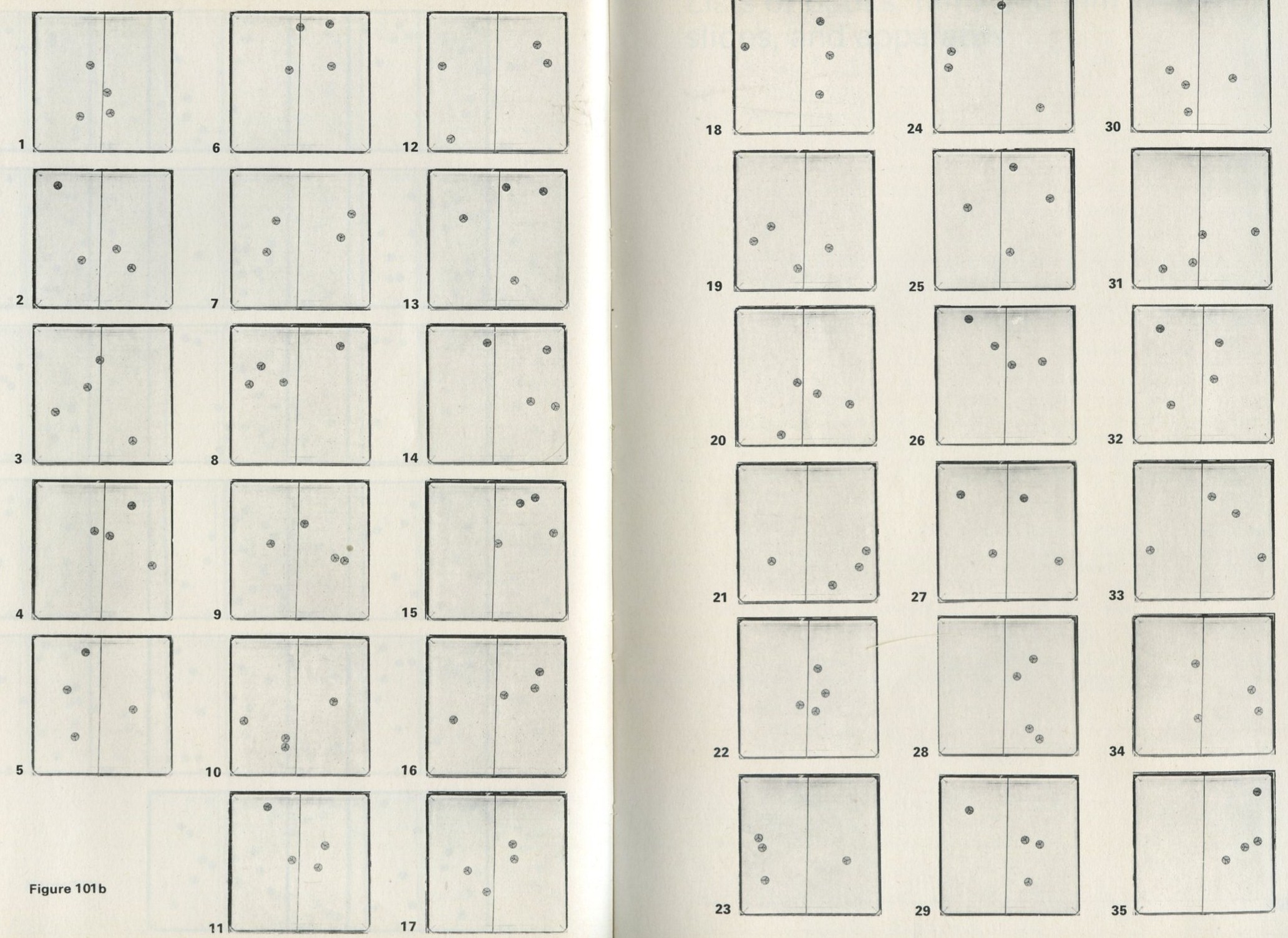
Figure 101b
Full Size Image
List of books, films and film loops, slides and apparatus
Books
Page numbers of references in this book are emphasised.
Books for students
Angrist, S. W., and Hepler, L. G. (1967) Order and chaos. Basic Books. 23, 26, 28. This is a valuable book but it may be thought too expensive for the use it will have in this Unit.
Carnot, S. (reprint 1960) Reflections on the motive power of fire. Dover. 155. This is a translated edition, first published in 1890 with additional papers by Clausius and Clapeyron, of Carnot's original work of 1824 entitled Refexions sur la puissance motrice du feu.
Ogborn, J. (1972) Nuffield Physics Special Molecules and motion. Penguin/Longman. 99.
PSSC (1968) College physics. Raytheon. 99.
PSSC (1965) Physics. 2nd edition. Heath. 99.
Rogers, E. M. (1960) Physics for the inquiring mind. Oxford University Press. 99.
Sandfort, J. F. (1964) Science Study Series No. 22. Heat engines. Heinemann. 155.
Ubbelohde, A. R. (1954) Man and energy. Penguin. 23, 26.
Books for teachers
Bent, H. A. (1965) The Second Law. Oxford University Press. A book which we strongly recommend to any teacher using the Unit. 3, 15, 133, 188.
Campbell, J. A. (1965) Why do chemical reactions occur? Prentice-Hall. A simple, empirical, and clearly explained account of chemical equilibrium. 140.
Gurney, R. W. (1949) Introduction to statistical mechanics. McGraw-Hill. The first two chapters contain one of the first, and one of the best, simple introductions to statistical mechanics. 188.
Millen, D. J. (ed.) (1969) Chemical energetics and the curriculum. Collins. Useful for the links it makes with chemistry teaching. 188.
PSSC (1968) College physics. Raytheon. This book (but not PSSC Physics) contains the very interesting PSSC treatment of thermodynamic ideas. 132.
Reif, F. (1967) The Berkeley Physics Course, Volume 5 Statistical physics. McGraw-Hill. A useful book for those who want access to the ideas of statistical mechanics worked out thoroughly and in detail. It is pretty tough going in places. 188.
Sherwin, C. W. (1961) Basic concepts of physics. Holt, Rinehart & Winston. This book, regrettably out of print, contains a good, clear, and simple introduction to the ideas of statistical mechanics which teachers would find helpful. 188.
Sources of physics teaching Part 1 (1966) Taylor & Francis. Contains articles from Contemporary physics. This volume includes two articles on the introduction of the Boltzmann distribution. 188.
Nuffield Advanced Chemistry (1970) Teachers' guide II. Penguin. 141.
Films and film loops
16 mm films
Change and chance: a model of thermal equilibrium in a solid. 13� minutes, black and white, silent. Penguin, XX1673. (Also available from Guild Sound and Vision Ltd.)
This computer-made film plays an essential part in the teaching of the Unit. It contains six short films on one reel, offered in this form rather than as 8 mm loops, for cheapness and clarity.
Random events 31 minutes, black and white, sound. Guild Sound and Vision Ltd, formerly Sound Services, 900 4116-5.
This PSSC film is not essential, but could prove a useful extra resource for the teaching of Part Three.
8 mm loops
'Forwards or backwards?' 1 Penguin, XX1668.
'Forwards or backwards?' 2 Penguin, XX1669.
'Forwards or backwards?' 3 Penguin, XX1670.
These three loops (in standard 8 only), produced for Nuffield Advanced Physics, play an important role in Part One of the Unit, though they could be replaced by other suitable film shown backwards.
Slides
The following is a list of slides for use with this Unit. They can be obtained from Penguin Books as a film strip under the title 'Unit 9 Change and chance', quoting the number XX1676.
9.1 World energy production and consumption
9.2 World fuel reserves
9.3 Total world rate of energy consumption
9.4 Cumulative world energy consumption
9.5 Total United Kingdom installed electrical generating power
9.6 Energy production. Africa
9.7 Energy production. North America
9.8 Growth of world population
9.9 Growth of number of cars in Britain
9.10 Energy account for cars
9.11 Power station with cooling towers (High Marnham)
9.12 Power station alongside a river (Belvedere)
9.13 The iodine molecular absorption spectrum
List of Apparatus
2B copper wire, 32 s.w.g. bare 9.6, 9.10, 9.14
9 Malvern energy conversion kit 9.1
12 two-dimensional kinetic model kit 9.2
27 transformer 9.7
42 lever arm balance 9.9, 9.10
44/1 G-clamp, large 9.10
44/2 G-clamp, small 9.1
52K crocodile clip 9.13, 9.15
59 l.t. variable voltage supply 9.9, 9.10
67 Bourdon gauge 9.11
70 demonstration meter 9.10
71/2 dial for demonstration meter, d.c. dial 5 A 9.10
71/10 dial for demonstration meter, d.c. dial 15 V 9.10
75 immersion heater 9.9, 9.10, 9.11
77 aluminium block 9.6, 9.10, 9.14
94A lamp, holder, and stand 9.7
132N thermistor (R S Components Ltd TH3) 9.13
133 camera 9.2
171 photographic accessories kit 9.2
176 1 2 volt battery 9.1, 9.6, 9.9, 9.11, 9.14
179 d.c. voltmeter (0-1 5 V) 9.11
191/2 fine grating 9.7
503-6 retort stand base, rod, boss, and clamp 9.7, 9.11, 9.13
507 stop watch or stop clock 9.11, 9.12
508 Bunsen burner 9.11, 9.13
510 gauze 9.11, 9.13
511 tripod 9.11, 9.13
512/1 beaker, 250 cm3
9.12, 9.13, 9.15
517 volumetric flask, 1 dm3 (1 litre) 9.12
522 Hoffmann clip 9.11
533 bucket 9.12
542 thermometer ( - 10 to 110�C) 9.6, 9.9, 9.11, 9.12, 9.13, 9.15
543 chinagraph pencil 9.11
548 round-bottomed flask 9.11
1001 galvanometer (internal light beam) 9.6, 9.10, 9.14, 9.15
1003/1 milliammeter (1 mA) 9.15
1003/2 milliammeter (10 mA) 9.13
1003/3 milliammeter (100 mA) 9.13
1003/5 ammeter (10 A) 9.9, 9.11
1004/1 voltmeter (1 V) 9.6
1004/2 voltmeter (10 V) 9.11
1004/3 voltmeter (100 V) 9.9
1005 multi-range meter (25 V range) 9.9
1023 solar motor 9.6, 9.14
1033 cell holder with U2 cells 9.1, 9.13, 9.15
1041 potentiometer holder 9.15
1051 Small electrical items
preset potentiometer, 5 kΩ 9.15
germanium transistor (e.g. OC 71) 9.13
1053 Local purchase items
card 9.6
counter 9.3, 9.4, 9.5, 9.8
piece of cork about 30 mm diameter� 10 mm thick 9.13
Polyfilla 9.15
Sellotape 9.10, 9.11
slab of expanded polystyrene 9.6, 9.10, 9.11
Vaseline 9.13
1054 Expendable items
constantan wire, 32 s.w.g., covered 9.6, 9.10, 9.14
copper wire, 14 s.w.g., bare 9.15
film, monobath combined developer-fixer 9.2
glass tube, 1 0 mm bore, 50 mm long 9.15
graph paper 9.3, 9.4, 9.8
piece of porous pot 9.11
rubber pressure tubing 9.11
1055 Small laboratory items
bung with two holes (for thermometer and T-piece) 9.11
burette 9.11
dice 9.3, 9.4, 9.5, 9.8
flat-bottomed flask, 1 dm3 (1 litre) 9.12
measuring cylinder, 100 cm3
9.10, 9.12
specimen tube 9.15
teat pipette 9.15
test-tube, hard glass, 150 mm by 25 mm, with cork 9.7, 9.11, 9.15
T-piece 9.11
1056 Chemicals
1 M copper sulphate solution 9.15
dextrose (glucose) 9.12
ethanol (ethyl alcochol) 9.12
formaldehyde 9.12
0.1 M hydrogen peroxide solution 9.12*
iodine crystals 9.7
methylene blue 9.12
phenolphthalein 9.12
0.1 M potassium iodide solution 9.12*
saturated potassium nitrate solution 9.15
0.1 M silver nitrate solution 9.15
silver wire 9.15
sodium hydroxide 9.12
sodium metabisulphite 9.12
sodium sulphite (anhydrous) 9.12
0.01 M sodium thiosulphate solution 9.12*
0.5 M sulphuric acid 9.1, 9.12*
0.2 % starch solution 9.12*
zinc dust 9.15
1064 low voltage smoothing unit 9.9, 9.10
1070 gas energy transfer apparatus 9.10
1072 semiconductor thermopile unit 9.14
* Alternative version.
Index