
The archaeologist hopes that he can define prehistoric societies and trace their development from the material remains they have left. His basic assumption is that the structure or pattern within the surviving material will reflect the structure of the societies that produced it. If he cannot show that he has recognised this structure in a rational way, his reconstruction of past events cannot be taken seriously.
At present there is a good deal of dissatisfaction among prehistorians with methods at their disposal for finding structure of this kind. One approach that is being investigated is to 'code' the material remains numerically and then to search for latent structure by suitable numerical procedures. It is already customary to describe some archaeological material quantitatively: for example, Early Stone Age assemblages of flint tools are regularly characterised by the relative proportions of the different tool types that they contain. It is only a small step, although not necessarily an easy one, to the analysis of this sort of descriptive data by numerical structure-seeking procedures.
As an archaeologist I have been interested to look for procedures that have been developed for similar classificatory problems in other subjects, especially in psychology. Since 1966, a number of likely multivariate procedures have been collected and, if necessary, adapted for use on the Chilton Atlas (all the programs mentioned in this summary are written in Atlas Algol).
At the same time, an attempt has been made to assess their potential value for archaeologists by testing them on two contrasting sets of actual data:
Programs so far tested on these sets of data at Chilton have been concerned with the following operations:
The above range of programs makes it possible to look at multivariate archaeological data in a number of different ways. The principal components and multidimensional scaling approaches provide a valuable indication of broad trends and structure. They indicate, for example, if there is a single, basic linear trend behind the material (which could result from development in time), or if there are simple, well-separated clusters (cf. fig. A).
However, for purely taxonomic purposes, a sound method of cluster analysis that could deal with large data matrices would be of great value. The average-link method illustrated on fig. B has shown reasonable results, but other possibilities are being investigated.
This work was carried out during tenure of a Senior Research Fellowship held jointly at the Chilton Atlas Laboratory and at Churchill College Cambridge. I would like to thank Dr. Howlett for making this project possible. I would also like to thank Professor D. G. Kendall and the staff of the Statistical Laboratory, 'Cambridge University, for their active co-operation.
1. F. R. Hodson, P.HA. Sneath and J. E. Doran, Biometrika 53,311,1966.
2. Le Paleolithique superieur en Perigord, D. de Sonneville-Bordes, Bordeaux, 1960.
3. P. Dempsey and M. B~umhoff, Amer. Antiq. 28, 496, 1963.
On diagrams A and B the 50 units represent 50 Palaeolithic occupation levels that have been described by the relative proportions of the different stone tool-types which they contain. Asterisks mark some levels that have produced a distinctive type of bone tool (split-based, bone points). This information is not used in the analyses, but provides a rough independent check on results: these sites are probably related and may be expected to cluster together on diagrams of this kind if the assumptions which lie behind the analyses are met.
The main groups suggested on both diagrams are labelled, and correspond more or less with a traditional archaeological grouping: A=Chatelperronian, B=Aurignacian, C/D=Gravettian.
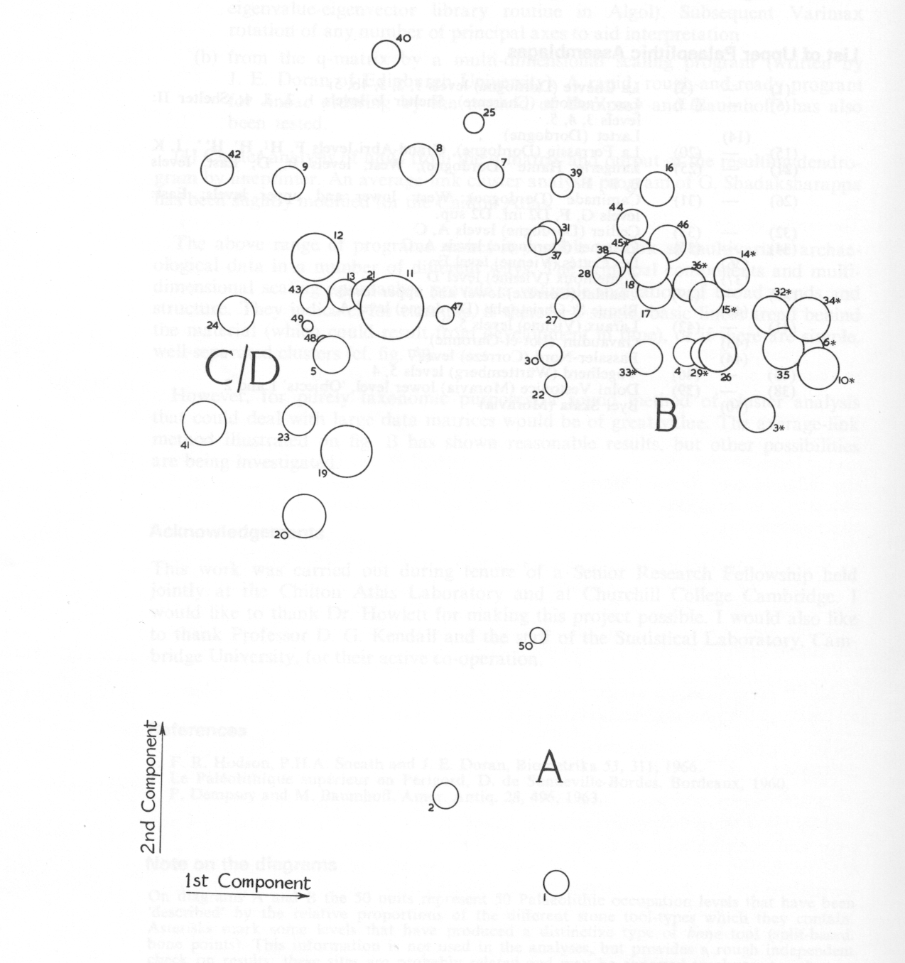
Projection of units (assemblages of stone tools) onto the first three principal axes or components. The first axis accounts for 20% of variation within the sample, the second for 12.5%, and the third (represented by the relative diameter of the circles) for 9.5%. The axes are located by eigenvectors of the r-matrix of correlations between variables (tool-types).
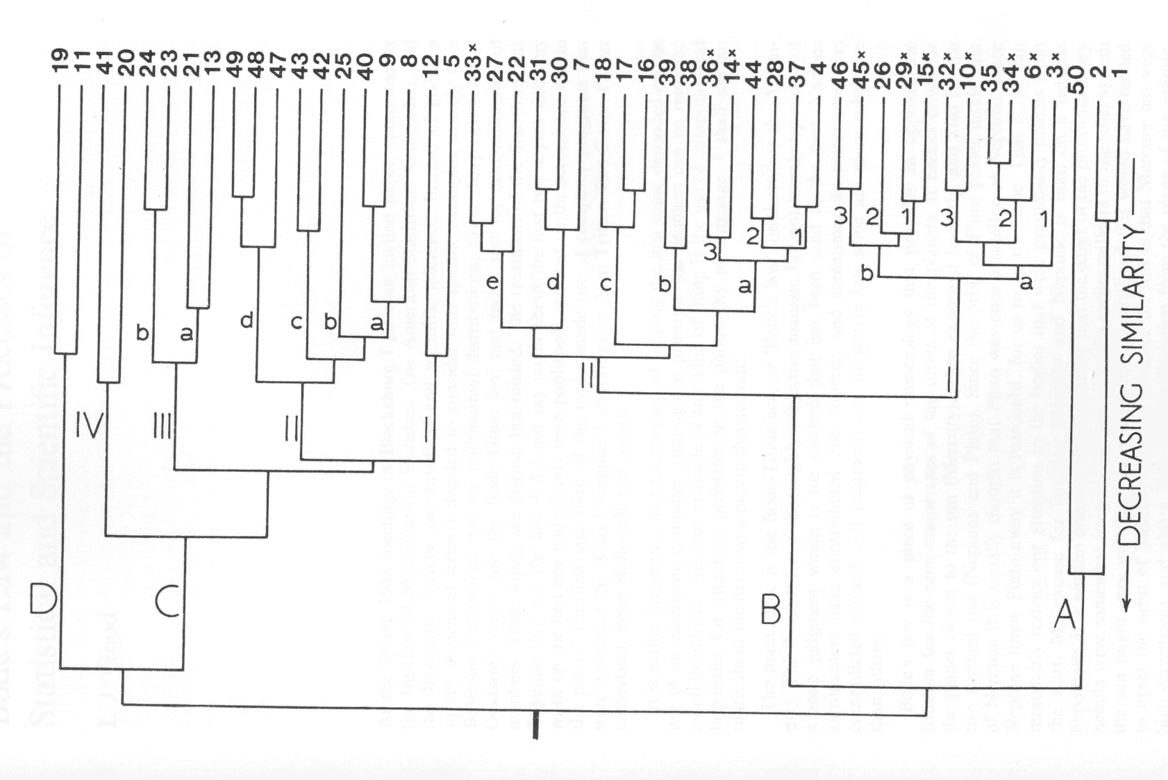
Unweighted Pair-Group Method from a q-matrix of Euclidean distances between assemblages, calculated from 46 variables, i.e. tool-types.
   (1)    -    (5)   La Chevre (Dordogne) levels 1, 2, 3, 4b, 5i
   (6)    -    (13)  Les Vachons (Charente), Shelter I: levels 1, 2, 3, 4;
                                             Shelter II: levels 3, 4, 5.
         (14)        Lartet (Dordogne)
  (15)    -    (20)  La Ferrassie (Dordogne), Grand-Abri levels F, H1, H', H'', J, K
  (21)    -    (25)  Laugerie Haute (Dordogne), West, levels B, D;
                                                East, levels B, B', F.
  (26)    -    (31)  Caminade (Dordogne), West: lower and upper levels;
                                          East: levels G, F, D2 info D2 sup.
  (32)    -    (33)  Cellier (Dordogne) levels A, C
  (34)    -    (35)  Castanet (Dordogne) levels A, C
         (36)        Les Cottes (Vienne) level E
         (37)        Fontenioux (Vienne) level D
  (37)    -    (39)  Chanlat (Correze) lower and upper levels
         (40)        Roque St-Christophe (Dordogne) level A
  (41)    -    (42)  Laraux (Vienne) levels 5, 3
         (43)        Gavaudun (Lot-et-Garonne)
         (44)        Bassaler-Nord (Correze) level 7
  (45)    -    (46)  Vogelherd (Wtirttemberg) levels 5, 4
  (38)    -    (39)  Dolni Vestonice (Moravia) lower level, 'Objects' 1 and 2
         (50)        Byci Skala (Moravia)
