Early attempts at computer animation in the UK in the period 1963 to 1975 were primarily via a batch computer that generated magnetic tapes for a microfilm recorder that processed the tapes and, instead of generating 35mm film and microfiche textual output, produced frames of line drawing output on 16mm film.
A Stromberg-Carlson SC4020 microfilm recorder was installed at AWRE Aldermaston in 1963 and used by Harwell, Culham and Aldermaston. By 1968, two other recorders were added. An SC4020 [11] was installed at the Atlas Computer Laboratory at Chilton (for use by the Rutherford High Energy Laboratory, Laboratory, Harwell Laboratory and university users). The BL120 [12] was installed at Culham mainly for their own use.
Output production was slow and primarily consisted of writing a computer program in FORTRAN, submitting it to a batch processing system on a mainframe computer that would generate a magnetic tape, waiting a day for output, then taking the magnetic tape to a microfilm recorder, often at a different location, viewing the resulting film or frames and repeating the process as the film was debugged. Despite this slow drawn out turnround, computer animated films were generated across a range of scientific disciplines in the period 1968-1973 (thermodynamics, quantum chemistry, chemical reactions, astrophysics, jet flow, meteorology etc).
As early as 1967, the BBC and the Open University (OU) explored the use of computer animation for educational programmes. One example, called Random Walk, was produced by Tony Pritchett and shown on the BBC in 1968.
In 1971, a more ambitious use of computer animation occurred with the Open University's first year Mathematics Course (M100-01). Each week, the aim was to have between 10 and 25 minutes of computer animated film to illustrate mathematical concepts. Two pilots were done at Culham (John Prior) and the Atlas Computer Laboratory (Bob Hopgood, Graham England and Bob Asbury). These trials indicated that it was feasible and the following weeks were produced mainly by Tony Pritchett and Jeffrey Lickess with the FORTRAN programs run on the University of London Atlas computer, debug frames plotted on a local Calcomp plotter and the final films produced on the SC4020 at the Atlas Computer Laboratory.
By 1972 it was clear that this production cycle was not ideal for the Open University work for several reasons:
See also P1: A Computer Graphics Facility for the Open University
The Open University had a 32K Data General Nova 16-bit mini-computer housed in the Technology Faculty which had the ability to connect to a variety of I/O devices and had a FORTRAN compiler so a system defined for that environment was a possibility. Access to peripherals included:
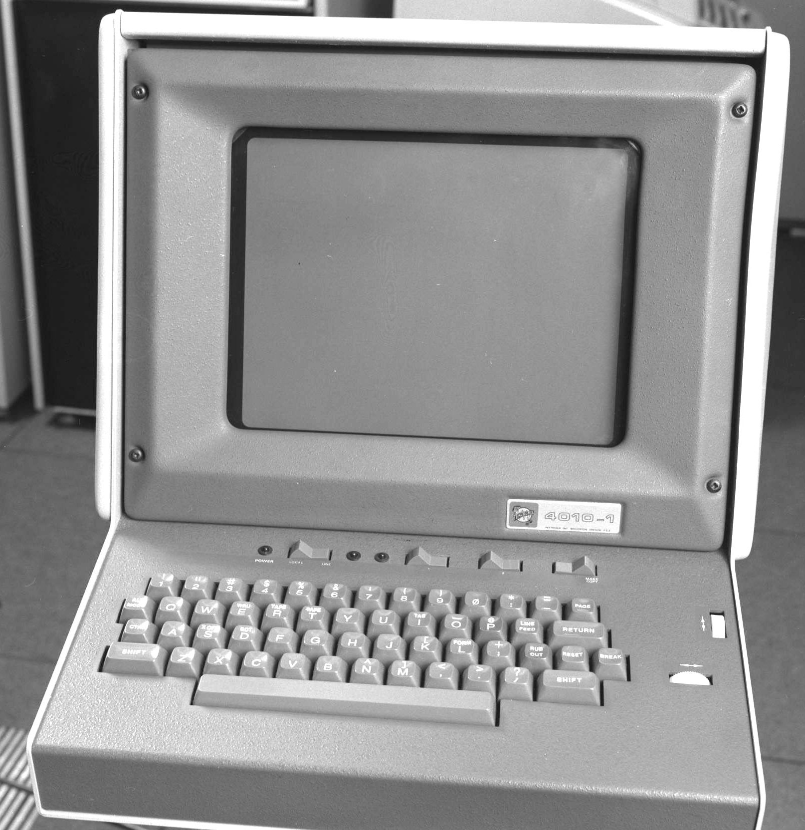
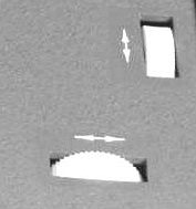
Probably the most relevant device was the storage tube. The 4010 could behave as both a standard teletype and a graphics device. In both modes, information displayed on the storage tube remained intact without the need for refreshing. In text mode, it could display 35 lines of 72 characters before the need to refresh the screen. In graphics mode it could output vectors to the screen in the address range (0,1023) in X and Y (only 768 were visible in the Y direction). For graphical input, the two thumbwheels (on the right of the keyboard) with cross-hairs displaying the cursor position on the display could be moved to point at a location on the screen and input the Y-coordinate followed by the X-coordinate together with the character pressed.
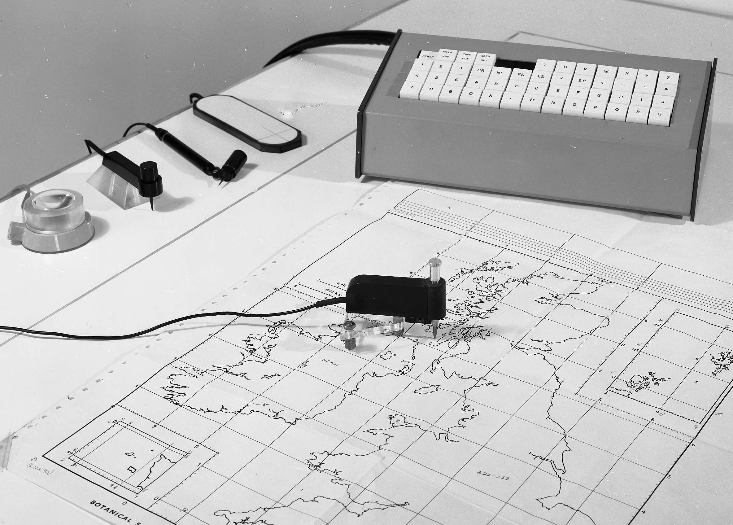
The D-MAC pencil follower was useful for tracing the outline of any diagrams needed. The coordinates of a position could be output and it was possible to add additional textual information to each scanned path.
Although aimed at the Data General Nova that existed at the OU, it was likely that additional computers would be purchased and there was a need to have a system not targeted specifically at the Nova.
The main reasons for each of these is:
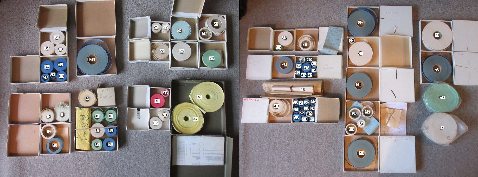
Sadly, Tony Pritchett passed away on the 28 August 2017. Kate Sullivan, a friend of Tony's, is providing a temporary home for Tony's archive. Scattered around the archive were many mentions of GRAM in various forms (hand-written notes, printed documents, computer output listings and paper tapes). Kate took on the job of scanning the documents relevant to GRAM and Terry Froggatt put together a system for reading paper tapes in a variety of formats.
Bob Hopgood and David Duce retyped significant parts of Kate's scans with the main problem being reading faint documents and mistyping.
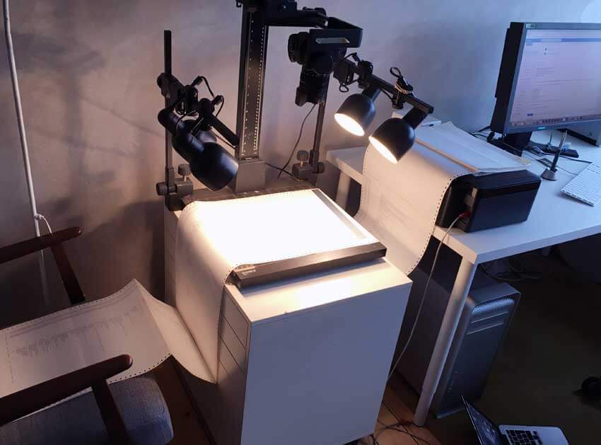
Between May 2020 and May 2021, Kate scanned about 1000 pages related to GRAM. Kate had managed to get an old rostrum stand to work as a scanning deck for the lineprinter output.
Early in 2021, Terry uploaded Tony's 75 paper tapes and found about 100 pages related to GRAM in the paper tapes, mainly listings of parts of GRAM, Most of Tony's tapes were 8-track, but there was one 5-track and one 7-track tape. and he converted these back to text files. Whereas it was unclear what documents related to other ones in the paper documents that Kate scanned, the paper tapes tended to look like transportation documents from one system to another or back-up copies of work in progress. Terry's input system is described in more detail in Appendix 5.
Bob and David took on the task of understanding what the GRAM system did and how it was constructed.
The system developed by Tony Pritchett, aimed initially at the OU Nova Computer, was called GRAM, that is GRAphic Macrogenerator. Tony was attracted by the flexibility of Christopher Strachey's General Purpose Macrogenerator (GPM) [1] as the basis for a system that could easily be changed to reflect the needs of the next task. GPM was originally intended as an intermediate language for the CPL programmming language for the Cambridge Titan computer.
He made the decision that the GRAM macroprocessor would be implemented using standard FORTRAN IV [2] to provide portability across mini computers. At the time, mini computers tended to have their own instruction set but were beginning to provide both FORTRAN and BASIC compilers, often with local extensions.
(Terry previously found a paper tape labelled GPM that was a version for the Elliott 903. See Resurrection Summer 2014.)
Most mini computers, like the Nova, at that time had 16-bit words and at most 32K words so memory was a limitation. The standard macro-generator tended to consist of an input string of symbols (characters) that generated one or more symbols in the output stream. For input symbols, GRAM was defined with two basic types, a character pair that fitted into a 16-bit word and a coordinate in the range -8191 to 8191 that also could be fitted into a single word.
Microfilm recorders at the time tended to have a display area in the range 0 to 1023. Scaling in GRAM was defined as a percentage so a SCALE of 6% was approximately the size of the output display area. This avoided the need for dealing with decimal fractions.
Early macrogenerators were frequently used primarily as a means of simplifying the writing of machine code programs. A macro with parameters could generate a sequence of machine code making it more readable and less prone to error. Similarly, macros defined in GRAM could be interpreted by GRAM. New macros could be added by the user to meet specific requirements for a particular animation.
Kate searched the archive of Tony's documents looking for anything related to GRAM and scanning these. This task was spread over the period of a year. In consequence, the information regarding GRAM was gradually added to over a long period. The findings were:
The main points coming out from the information available:
The long period between the first and last download meant that many of the decisions that were made were taken with only partial understanding of the GRAM system.
Our main objective was to recover a working GRAM implementation that could be enhanced to generate animated SVG output as a substitute for the output devices current at the time GRAM was written.
Near the end of January 2021 we had a reasonably complete listing of the 1906A Nova GRAM FORTRAN code and David attempted to compile it with the GNU FORTRAN system running on MacOS. Somewhat later Bob managed to get a version of the Silverfrost compiler to work on his Windows PC. Both were a reasonably complete implementation of FORTRAN IV. Silverfrost was quite precise in what it regarded as a correct program and came up with many more warnings and potential errors than the GNU FORTRAN. On the other hand the GNU FORTRAN tended to be more flexible in what could be done.
The GNU FORTRAN compiler conforms to FORTRAN 95, 2003 and 2008. Silverfrost FORTRAN conforms to FORTRAN 95. We were careful to keep the code as close to the original dialect of FORTRAN as possible and avoided the use of more recent features, such as more flexible output formatting and control structures. The two minor exceptions we made to this were the use of ADVANCE="NO" with WRITE statements generating SVG markup so that lists of coordinates were output on a single line and the FORTRAN 90 ISHFT bit shifting function used in the input and output routines for character manipulation.
Progress was quite slow early on for a variety of reasons:
For this reason, in February 2021 David and Bob changed direction and concentrated on getting the earlier 1973 Nova version to work. At least that would give some confidence in how the macro system worked with the ability to generate drawings, originally to be shown on the Tektronix 4010, as SVG diagrams. David had the best understanding of how the macrogenerator worked and managed to demonstrate many of the examples used by Tony in his GRAM macroprocessor introduction.
By March 2021, David and Bob moved to looking at a fuller version aimed at the Chilton PRIME 400 but this turned out to be incomplete and was later abandoned.
The final choice in late March 2021 was to take the later 1977 code aimed at the Nova as the basis for getting a version to work. This was one of the paper tapes that Terry had read in and listed, It dated from about 17/5/77. Not all routines were of that age but most were.
By now, it had been decided that:
This 1977 Nova code was the version of GRAM that was used from March onwards. At that stage, David had a good idea of how the macro stack worked but less understanding of the set of primitives used by this GRAM version.
Also multiple versions of the macros defining the GRAM Editor and the graphic animation features meant that it was not obvious which, if any, of the many sets of each applied to the FORTRAN code that had been compiled.
The attempts to get this code to work were driven by simple examples such as:
(DEF A #1)
(A "ABC")
(DEF TEN 10)(DEF ONE 1)(DEF SIXTY 60)(DEF EIGHTY 80)
(TEN) (ONE) (SIXTY) (EIGHTY)
It was possible to change the name DEF to something else and frequently below you will see a colon in place of DEF.
This version of GRAM had a different input syntax to Strachey's original GRAM, but there were strong similarities in the structure of the implementation, although the NOVA version was written in FORTRAN. The FORTRAN COMMENT statement was used sparingly to say the least! Much of the code was concerned with stack and index manipulation.
Studying this version enabled us to gain a basic understanding of how the code was working and in particular how the single stack represented by a pair of arrays LIST and LNK with the latter storing pointers (array indices) and the former pointers or values of the other datatypes, character pairs and integer values. An example of the stack layout we discerned is shown below.
At the time this work was done, and indeed until we were in the process of writing this paper, we had not come across a set of papers on GPM in Resurrection by Andrew Herbert, on the Elliott 903 version (deriving from a paper tape in Terry Froggatt's collection), P.A. Cherapanov a port to C, Bob Eager ML/1 - Son of GPM? and Andrew Herbert on Elliott 905 ML/I. Andrew Herbert's first paper references a BCPL implementation by Martin Richards at Cambridge. The remark in Herbert's paper:
is interesting as the FORTRAN version also used a single stack. There were times we wished Tony had used two stacks rather than one and indeed the explanation of the Mechanism of Evaluation suggests that more than one storage area would have been appropriate. Perhaps the structure of the implementation was driven by a desire not to deviate too much from the original GPM or memory considerations at the time the first implementation was written.
It is worth repeating the comments made by Tony in P3: GRAM: A Macrogenerator for Computer Graphics.
GRAM is basically an adaptation of Christopher Strachey's General Purpose Macrogenerator [1] to handle graphics more efficiently. It also bears a generic resemblance to some other stack-based languages.
GPM is a character-stream processor: its primitive symbol is a single alphanumeric character. Macro names are held internally as character strings, which necessitates a linear search down the list of names each time a macro is called. GPM therefore has a reputation of being extremely slow in execution, which was not a very important consideration in the application for which it was originally intended, i.e. implementing a CPL compiler.
There are three main ways in which GRAM differs from GPM, which were made primarily to improve efficiency for interactive graphics:
There are three ways in which the GRAM system could be, and was, extended.
The set of built-in primitives in this early version of GRAM was very small. There were no specific primitives for generating graphical output, though graphic input and output mode were available and input could be taken from different source devices. We did make some extensions to add a capability to generate SVG output, both by defining new macros and new primitives, but that was purely as a learning exercise. At this point we decided to halt exploration of this version and look at a later version which seemed to offer promise, both in terms of relative completeness and capabilities. As this was the limit of our detailed exploration, we refer to this as the "final" version.
This turned out to be the final version we have explored in detail. As described in more detail in Tony's draft thesis submission 5.1 The GRAM Item, four types of item were used.
External syntax: A string of up to four decimal digits (0-9) optionally preceded by a minus sign.
Example:
1234   -99   0   430   -8
Internal form: An integer in the range -8191 to +8191. The limitation on range is in order to distinguish numbers from the other three types internally, which are represented by integers outside this range.
External syntax: One or two characters out of the whole ASCII graphic character set (apart from ", but including space) surrounded by string quotes ".
Example:
"AZ" "5" "**" "!?" "." ",H"
Internal form: Two characters packed into an integer word left to right. In the case of only one character externally, the least significant byte is a blank (all zeros). Provided the characters are held externally as two 8-bit ASCII bytes out of the graphic range (ie not control characters), they will always form an integer greater than 8191.
Pairs of string quotes between contiguous alpha-pair items may be omitted in input, and are always omitted in output:
"ABCDEFG" is equivalent to "AB""CD""EF""G"
Note that if the string quotes contain an odd number of characters, the last item always contains the odd integer single character.
External syntax:
(a) A string of characters from the range of letters A-Z and numerals 0-9 but always starting with a letter
Example:
ABC THING M45 X ZOOLOGICAL
The number of characters in a name is only limited by the maximum length of the input line (typically 72).
(b) Any other single character out of the ASCII graphic subset which is not a Control Symbol or syntactic device.
* + - / ? % & are all valid Names
Internal form: A pointer to an entry in a table, added to a negative constant to keep it less than -8191 in order to distinguish it from other types.
The table contains (a) the characters defining the external form of the name, and (b) a pointer to a corresponding Macro Body, if one has been defined for it.
External syntax: One of the following characters:
< > ( ) # !
Internal form: A large negative integer outside the range occupied by Names.
These items have special control functions, eg delimiting a macro call: (NAME ARG1 ARG2).
A significant change here was that the first version had a string item type, where a string was represented by a sequence of pairs of characters and a terminator. Here strings were replaced by pairs of characters. One implication of this was that a string "ABCD" presented as a macro parameter would be mapped to two parameters, "AB" and "CD". The significance of this took a while to dawn! In this final version the set of control symbols was extended beyond the set listed above.
The original NOVA code was structured into a set of overlays as shown in the figure below. This was interesting in terms of the grouping of routines, but was redundant for current hardware/software environments and was discarded.
The diagram below shows the calling tree of subroutines/ functions in the code and assigns them to a set of categories. Working out this tree was very helpful in understanding the code and the purpose of each routine.
The main points about the structure of the implementation are as follows:
Rather than attempting to describe the implementation in detail, we halt the description at this point and in the next section consider a set of examples that illustrate the way this version of GRAM operates.
The aim of this section is to give a flavour of the internal workings of the "final" version of GRAM through a set of examples. It is not intended as a GRAM tutorial; for that purpose the reader is referred to the (incomplete) GRAM Manual, though this comes with a warning that not all of this may refer to this "final" version of GRAM and the associated set of macros.
Consider a simple example.
PRIM : 28
PRIM STOP 100
PRIM PRMACS 103
:A 1
:B [#1]
B(A)
PRMACS
STOP
This associates names, ":", "STOP" and "PRMACS" with primitives numbers 28, 100 and 103 respectively. The first is used to define a new macro (previously DEF was used), the last to print out the names of macros stored and various pointers.
The input line is processed by the subroutines INPUT and ALFIN, the latter essentially parsing the input line. For the first line, the input line and resulting input buffer are shown below.
PRIM : 28
  -32764  -13191   -8196      28  -32763  -32761  -32760
GRAM has essentially two modes, one in which brackets around macro invocations are expected, e.g. (PRIM : 28) and one in which brackets may be omitted by the user and inserted by the INPUT routine. INPUT here is used in this latter mode, so the first entry in the buffer, -32764, represents "(" and a matching ")" (-32763) is at position 5. Special characters are converted to integer values as shown below.
| Symbol | Representation |
|---|---|
| < | -32766 |
| > | -32765 |
| ( | -32764 |
| ) | -32763 |
| # | -32762 |
| ^ | -32761 |
| ; | -32760 |
The final two words in the buffer are terminators.
The name PRIM is recognised as a macro name. ALFIN searches the stack (using the search chain which is explained later) for this name. If it is not found, the name is inserted in the stack. In this case PRIM is a built-in name and the value -13191 references this. The value is computed as -(4999+8192). The value 8192 is a reserved value and 4999 is the position on the stack where PRIM is defined.
The stack in GRAM consists of two integer arrays, LIST and LNK. The latter holds pointers to other cells and the former holds either values or pointers. Various variables point to locations in the stack. Apart from the top of the stack which holds the definition of PRIM, the stack is initialised so that each cell points to the next cell.
ALFIN then searches for ":" on the stack. As this is a new name a stack entry is created, at position 3 (which stores the name ":") and the buffer stores the value -8196 which is -(4+8192), one stack position after the name.
The main loop then calls subroutine LOAD which either loads values onto the stack or outputs values. In this case values are loaded onto the stack so the stack will then hold 14828 (in hex 3A00) which is the character ":" in the MSB and zero in the LSB.
| I | 1 | 2 | 3 | 4 | 5 | 6 | 7 | 8 | 9 | 10 | 11 | 12 | 13 | 14 | 15 | 16 | 17 | 18 | 19 | 20 |
|---|---|---|---|---|---|---|---|---|---|---|---|---|---|---|---|---|---|---|---|---|
| LIST(I) | 0 | 4996 | 14848 | 2 | 0 | 0 | 0 | 0 | 0 | 0 | 0 | 0 | 0 | 0 | 0 | 0 | 0 | 0 | 0 | 0 |
| LNK(I) | 5 | 3 | 4 | 0 | 6 | 7 | 8 | 9 | 10 | 11 | 12 | 13 | 14 | 15 | 16 | 17 | 18 | 19 | 20 | 21 |
The value in cell 4 points to cell 2 which in turn points to the previous name starting in cell 4996 (PRIM).
After the values in the input buffer have been copied to the cells, the stack is:
| I | 1 | 2 | 3 | 4 | 5 | 6 | 7 | 8 | 9 | 10 | 11 | 12 | 13 | 14 | 15 | 16 | 17 | 18 | 19 | 20 |
|---|---|---|---|---|---|---|---|---|---|---|---|---|---|---|---|---|---|---|---|---|
| LIST(I) | 0 | 4996 | 14848 | 5 | 2 | -13191 | -8196 | 28 | 0 | 0 | 0 | 0 | 0 | 0 | 0 | 0 | 0 | 0 | 0 | 0 |
| LNK(I) | 6 | 3 | 4 | -28 | 0 | 7 | 8 | 9 | 10 | 11 | 12 | 13 | 14 | 15 | 16 | 17 | 18 | 19 | 20 | 21 |
The main loop then calls subroutine NEXT to identify the next cell to process in either the input buffer or the stack (depending on the value of a variable LS). The action of the main loop depends on the value IW returned by NEXT, which includes stacking a call, executing a call, loading an argument, processing a primitive, processing a user-defined primitive and STOP. Without going into details, after the main loop has processed the first line of input the stack has the following form:
| I | 1 | 2 | 3 | 4 | 5 | 6 | 7 | 8 | 9 | 10 | 11 | 12 | 13 | 14 | 15 | 16 | 17 | 18 | 19 | 20 |
|---|---|---|---|---|---|---|---|---|---|---|---|---|---|---|---|---|---|---|---|---|
| LIST(I) | 0 | 4996 | 14848 | 5 | 2 | -13191 | -8196 | 28 | 0 | 0 | 0 | 0 | 0 | 0 | 0 | 0 | 0 | 0 | 0 | 0 |
| LNK(I) | 6 | 3 | 4 | -28 | 0 | 7 | 8 | 9 | 10 | 11 | 12 | 13 | 14 | 15 | 16 | 17 | 18 | 19 | 20 | 21 |
The stack frame for ":" is cells 2 to 5. (The value in LNK(1) at this point, 6, points to the next free cell in the stack.) Cell 2 is a pointer to the previous macro definition on the stack (the reserved macro PRIM at the top of the stack). Cell 3 is the name of the macro and cell 4 points to the macro body. The negative value, -28, indicates that this is a built-in function, number 28. The LIST value for cell 5 points back to the start of the macro definition and the LNK value, 0, indicates the end of the definition.
In a similar way, interpretation of the next two input lines PRIM STOP 100 and PRIM PRMACS 103 leads to the following stack (where the second row (LIST) prints cell values in hex):
| I | 1 | 2 | 3 | 4 | 5 | 6 | 7 | 8 | 9 | 10 | 11 | 12 | 13 | 14 | 15 | 16 | 17 | 18 | 19 | 20 |
|---|---|---|---|---|---|---|---|---|---|---|---|---|---|---|---|---|---|---|---|---|
| LIST(I) | 0 | 4996 | 14848 | 5 | 2 | 2 | 21332 | 20304 | 10 | 6 | 6 | 20562 | 19777 | 17235 | 16 | 11 | -13191 | -8207 | 103 | 0 |
| LIST(I) | 0 | 1384 | 3A00 | 5 | 2 | 2 | 5354 | 4F50 | A | 6 | 6 | 5052 | 4D41 | 4353 | 10 | B | CC79 | DFF1 | 67 | 0 |
| LNK(I) | 17 | 3 | 4 | -28 | 0 | 7 | 8 | 9 | -100 | 0 | 12 | 13 | 14 | 15 | -103 | 0 | 18 | 19 | 20 | 21 |
Cells 7 and 8 contain the characters "ST" "OP" and 12, 13, 14 "PR" "MA" "CS". The function values are in cells 9 and 15. The chain of cells used for finding names on the stack now runs through cells 11, 6, 2 and 4996. The next free cell is 17.
The next input line
:A 1
defines the macro A to have the value 1. Processing this input line proceeds in a similar way and after execution of the definition the stack contains:
| I | 1 | 2 | 3 | 4 | 5 | 6 | 7 | 8 | 9 | 10 | 11 | 12 | 13 | 14 | 15 | 16 | 17 | 18 | 19 | 20 |
|---|---|---|---|---|---|---|---|---|---|---|---|---|---|---|---|---|---|---|---|---|
| LIST(I) | 0 | 4996 | 14848 | 5 | 2 | 2 | 21332 | 20304 | 10 | 6 | 6 | 20562 | 19777 | 17235 | 16 | 11 | 11 | 16640 | 25 | 0 |
| LIST(I) | 0 | 1384 | 3A00 | 5 | 2 | 2 | 5354 | 4F50 | A | 6 | 6 | 5052 | 4D41 | 4353 | 10 | B | B | 4100 | 19 | 0 |
| LNK(I) | 20 | 3 | 4 | -28 | 0 | 7 | 8 | 9 | -100 | 0 | 12 | 13 | 14 | 15 | -103 | 0 | 18 | 19 | 23 | 21 |
| I | 21 | 22 | 23 | 24 | 25 | 26 | 27 | 28 | 29 | 30 | 31 | 32 | 33 | 34 | 35 | 36 | 37 | 38 | 39 | 40 |
|---|---|---|---|---|---|---|---|---|---|---|---|---|---|---|---|---|---|---|---|---|
| LIST(I) | -8196 | -8211 | 1 | -32760 | 17 | 0 | 0 | 0 | 0 | 0 | 0 | 0 | 0 | 0 | 0 | 0 | 0 | 0 | 0 | 0 |
| LIST(I) | DFFC | DFED | 1 | 8008 | 11 | 0 | 0 | 0 | 0 | 0 | 0 | 0 | 0 | 0 | 0 | 0 | 0 | 0 | 0 | 0 |
| LNK(I) | 22 | 26 | 24 | 25 | 0 | 27 | 28 | 29 | 30 | 31 | 32 | 33 | 34 | 35 | 36 | 37 | 38 | 39 | 40 | 41 |
The representation of A starts in cell 17 with a pointer in LIST(17) to the previous cell in the FIND chain. This chain is used by the subroutine FIND to locate macro names on the stack. Cell 18 holds the macro name, A. The value in cell 19 points to the end of the macro definition, cell 25, which in turn points back to the start of the macro definition through the LIST value, 17, and denotes the end of the definition by the LNK value 0. The LNK value of cell 19 points to the macro body, in this case the numerical constant 1, in cell 23. The value in cell 24, -32760, marks the end of the macro body.
It is interesting to note how the stack has become fragmented. The next free cell pointer in cell 1, points to cell 20, which together with cells 21 and 22 contain values that were generated in the processing of the input line but are no longer needed. Cell 22 points to cell 26 which is the start of the region of the stack that has not yet been used. Stack fragmentation can make it "interesting" to trace the execution of a statement.
The next input line is the first example of the definition of a macro with a body that is neither a built-in primitive, nor a constant. In this case the macro returns the value of its first argument, #1.
:B [#1]
The symbols "[" and "]" are shorthand for "(<" and ">)" and are expanded as such by ALFIN. The effect of "<" and ">" is to protect the body of the macro from evaluation in the definition phase. After the input line has been processed the stack contains:
| I | 1 | 2 | 3 | 4 | 5 | 6 | 7 | 8 | 9 | 10 | 11 | 12 | 13 | 14 | 15 | 16 | 17 | 18 | 19 | 20 |
|---|---|---|---|---|---|---|---|---|---|---|---|---|---|---|---|---|---|---|---|---|
| LIST(I) | 0 | 4996 | 14848 | 5 | 2 | 2 | 21332 | 20304 | 10 | 6 | 6 | 20562 | 19777 | 17235 | 16 | 11 | 11 | 16640 | 25 | 17 |
| LIST(I) | 0 | 1384 | 3A00 | 5 | 2 | 2 | 5354 | 4F50 | A | 6 | 6 | 5052 | 4D41 | 4353 | 10 | B | B | 4100 | 19 | 11 |
| LNK(I) | 26 | 3 | 4 | -28 | 0 | 7 | 8 | 9 | -100 | 0 | 12 | 13 | 14 | 15 | -103 | 0 | 18 | 19 | 23 | 21 |
| I | 21 | 22 | 23 | 24 | 25 | 26 | 27 | 28 | 29 | 30 | 31 | 32 | 33 | 34 | 35 | 36 | 37 | 38 | 39 | 40 |
|---|---|---|---|---|---|---|---|---|---|---|---|---|---|---|---|---|---|---|---|---|
| LIST(I) | 16896 | 34 | 1 | -32760 | 17 | 0 | -8196 | -8214 | -32764 | -32762 | 1 | -32763 | -32760 | 20 | 0 | 0 | 0 | 0 | 0 | 0 |
| LIST(I) | 4200 | 22 | 1 | 8008 | 11 | 0 | DFFC | DFEA | 8004 | 8006 | 1 | 8005 | 8008 | 14 | 0 | 0 | 0 | 0 | 0 | 0 |
| LNK(I) | 22 | 29 | 24 | 25 | 0 | 27 | 28 | 35 | 30 | 31 | 32 | 33 | 34 | 0 | 36 | 37 | 38 | 39 | 40 | 41 |
Recall that the first free cell in the stack after the previous input had been processed was cell 20. Accordingly, the definition of B starts in cell 20 which contains the pointer to the previous cell in the FIND chain. Cell 21 contains the name of the macro, "B", and the value in cell 22 points to the end of the macro (34) whilst the link, 29, points to the start of the macro body. The values here, -32764, ...-32763, -32760 correspond to (#1) and an end marker. As usual the last cell, 34, has a value that points to the start of the macro definition (20) and a link value of 0 denoting end of macro.
The final line in this small example executes the macro B, with a parameter which is the result of executing A.
B(A)
Without going into the details:
(B(A))
Consider the following code which generates a single triangle shape, using primitive functions defined in GRAM.
PRIM : 28
PRIM NUTR 61, PRIM DNTR 62, PRIM UPTR 63, PRIM FIG 64
PRIM ROT 67
PRIM EXTR 91
PRIM STOP 100
PRIM PRMACS 103
:TRIANGLE 4!0 4000 2000 -4000 -2000 -4000 0 4000
NUTR,DNTR,FIG TRIANGLE,UPTR,EXTR(1)
PRMACS
STOP
This generates the output shown below. The area shown is from -8000 to 8000 in the X and -6000 to 6000 in the Y.
The basic idea is to build a tree structure representing the line graphics, including, as we will see shortly, transformations, then traverse this to generate graphical output. The output routine (GDRAW) in GRAM has been modified to generate Scalable Vector Graphics (SVG) markup; the source code originally targetted a Tektronix storage tube as output device. As before the PRIM statements associate symbolic names with the built-in primitive functions, the exception being 103 which is a user-defined extension to print out the locations of macros on the stack.
:TRIANGLE defines a macro, TRIANGLE, which holds a list of 2D coordinates. The first number, 4, is the number of coordinates in the list and "!" is a null-character separator. The output generated by PRMACS shows the location of the macros on the stack.
I       BODY  START MACRO NAME
    47    56    48  TRIANGLE
    41  -103    42  PRMACS
    36  -100    37  STOP
    31   -91    32  EXTR
    26   -67    27  ROT
    18   -64    19  FIG
    14   -63    15  UPTR
    10   -62    11  DNTR
     6   -61     7  NUTR
     2   -28     3  :
  4996   -30  4997  PRIM
TRIANGLE is stored in the stack beginning at cell 47. To make the definition easier to follow, the LIST values of unrelated cells have been removed in the decimal representation of LIST.
| I | 41 | 42 | 43 | 44 | 45 | 46 | 47 | 48 | 49 | 50 | 51 | 52 | 53 | 54 | 55 | 56 | 57 | 58 | 59 | 60 |
|---|---|---|---|---|---|---|---|---|---|---|---|---|---|---|---|---|---|---|---|---|
| LIST(I) | 41 | 21586 | 18753 | 20039 | 19525 | 67 | 4 | -32759 | 0 | 4000 | 2000 | |||||||||
| LIST(I) | 24 | 5052 | 4D41 | 4353 | 2E | 29 | 29 | 5452 | 4941 | 4E47 | 4C45 | 43 | 0 | DFD3 | 0 | 4 | 8009 | 0 | FA0 | 7D0 |
| LNK(I) | 42 | 43 | 44 | 45 | -103 | 0 | 48 | 49 | 50 | 51 | 52 | 56 | 54 | 55 | 68 | 57 | 58 | 59 | 60 | 61 |
| I | 61 | 62 | 63 | 64 | 65 | 66 | 67 | 68 | 69 | 70 | 71 | 72 | 73 | 74 | 75 | 76 | 77 | 78 | 79 | 80 |
|---|---|---|---|---|---|---|---|---|---|---|---|---|---|---|---|---|---|---|---|---|
| LIST(I) | -4000 | -2000 | -4000 | 0 | 4000 | -32760 | 47 | 0 | 0 | 0 | 0 | 0 | 0 | 0 | 0 | 0 | 0 | 0 | 0 | |
| LIST(I) | F060 | F830 | F060 | 0 | FA0 | 8008 | 2F | DFD9 | 0 | 0 | 0 | 0 | 0 | 0 | 0 | 0 | 0 | 0 | 0 | 0 |
| LNK(I) | 62 | 63 | 64 | 65 | 66 | 67 | 0 | 69 | 70 | 71 | 72 | 73 | 74 | 75 | 76 | 77 | 78 | 79 | 80 | 81 |
The string "TRIANGLE" is contained in cells 48 to 51. The number of coordinate points, 4, is stored in cell 56; cell 57 is a separator represented as -32759, and the values of the coordinates are in cells 58 to 65. The value -32760 in cell 66 marks the end of the macro body and the value 47 in cell 67 is a link back to the start of the macro definition and the link, 0, marks the end of the macro. Note how the coordinate values are stored as integers, one per cell.
Now consider the line
NUTR,DNTR,FIG TRIANGLE,UPTR,EXTR(1)
which consists of 5 primitive functions, separated by commas. Roughly speaking, NUTR starts a new tree, DNTR starts a new level, UPTR, goes back a level, FIG inserts a reference to the data defining a figure and EXTR traverses the tree. The parameter (1) to EXTR is related to the frame number to display. These primitives are implemented in GRAM by the subroutine TOTREE which takes a single argument, M, a number corresponding to the function to perform. In this case the trace of TOTREE is
TOTREE: ENTERED M=     1
TOTREE: ENTERED M=     2
TOTREE: ENTERED M=     4
TOTREE: ENTERED M=     3
These values correspond to NUTR, DNTR, FIG and UPTR. TOTREE creates a linear representation of the tree in an array, MA. After the final execution of TOTREE, MA contains
2 4 9 4 56 3
We will ignore for the moment the second and third elements. The elements highlighted in red, 2, 4, 3 correspond to the M values above. The FIG macro has a parameter, TRIANGLE, which contains the coordinates of the points of the lines in the figure. As seen above, 56 is the start address of the body of TRIANGLE.
The primitive EXTR is implemented by the subroutine EXTREE which effectively traverses the tree represented by the array MA. Ignoring DNTR and UPTR for the moment, traversal of the pair 4, 56, essentially calls subroutines GROUT and GRDRAW which generate the graphical output, in this case SVG path elements. The output generated in this case is the path element:
<path d="M 0, 4000L 2000, -4000L -2000, -4000L 0, 4000"/>
The part that has been glossed over in this explanation is the way the coordinate transformation that is applied to the coordinates is calculated. In this case the transformation is the identity transformation, but it is perhaps easier to see what is happening by considering the addition of a rotation transformation. To apply a -90 degree transformation, the input would be:
NUTR,DNTR,FIG TRIANGLE,ROT -90,UPTR,EXTR(1)
The SVG path element and output generated are shown below.
<path d="M 4000, 0L -4000, -1999L -3999, 2000L 4000, 0"/>
The trace to TOTREE is now:
TOTREE: ENTERED M=     1
TOTREE: ENTERED M=     2
TOTREE: ENTERED M=     4
TOTREE: ENTERED M=     7
TOTREE: ENTERED M=     3
M=7 corresponds to the rot primitive. The linear representation of the tree now has the form:
2 4 9 4 56 3 12 3
The first three entries 2, 4, 9, correspond to DNTR. The value 9 is a pointer to the next free element in the array. The value 4 points to the element in array where this level starts.
Skipping over the details, TOTREE computes a transformation matrix for each level in the tree which is stored in an array of 240 elements. Since each array has 12 elements, this allows for up to 20 matrices to be stored. In this instance, TOTREE generates two matrices, an identify matrix for the top of the tree and a matrix representing the rotation to apply to the TRIANGLE. The matrix stack is shown below with a blank line inserted to separate the two matrices. The first 3 rows in each matrix are a 3x3 matrix representing scaling and rotation, the 4th row represents translations.
    1.00    0.00    0.00
    0.00    1.00    0.00
    0.00    0.00    1.00
    0.00    0.00    0.00

   -0.00   -1.00    0.00
    1.00   -0.00    0.00
    0.00   -0.00    1.00
    0.00   -0.00    0.00
So in this case the pair of entries in the tree, 12, 3, indicate the type of transformation to apply (3) and the starting point of the transformation in the stack (12). (The previous entry, 3, corresponds to UP a level.) If we were to add a MOVE transformation after the rotation (MOVE is primitive 65)
NUTR,DNTR,FIG TRIANGLE,ROT -90,MOVE 1000 1000,UPTR,EXTR(1)
the matrix stack changes to:
    1.00    0.00    0.00
    0.00    1.00    0.00
    0.00    0.00    1.00
    0.00    0.00    0.00

   -0.00   -1.00    0.00
    1.00   -0.00    0.00
    0.00   -0.00    1.00
 1000.00 1000.00    0.00
and without the rotation, the linear representation of the tree and matrix stack are:
2 4 9 4 61 3 12 1
    1.00    0.00    0.00
    0.00    1.00    0.00
    0.00    0.00    1.00
    0.00    0.00    0.00

    1.00    0.00    0.00
    0.00    1.00    0.00
    0.00    0.00    1.00
 1000.00 1000.00    0.00
(Adding the definition of MOVE changes the start address of the coordinates of TRIANGLE from cell 56 to 61.) The type of the transformation has changed from 3 to 1 (the final element in the array). Rather than do general matrix multiplications to apply a transformation matrix to a set of coordinates, GRAM identifies special cases that only require a restricted set of the matrix elements and hence reduces the number of multiplications and additions required, which might well have resulted in a valuable performance improvement at the time.
When transformations are considered, EXTREE now has to determine the transformation matrix to apply at each level in the tree. Again skipping over the details, essentially this will be the composition of the matrix at the current level with the matrices higher up the tree to create an accumulated matrix and again, presumably to save execution time, GRAM does not do general matrix multiplications, but uses the types of the matrices to work out the specific elements that need to be combined. Knowing where the coordinates of a figure are located on the stack, EXTREE then invokes the subroutine MATRIX to apply the accumulated transformation matrix and finally the subroutine GROUT generates the graphical output.
Suppose we want to draw multiple shapes, specifying a rotation for each. Rather than write out the primitive invocations in full, we could define a macro, say, DISP with two parameters, the name of the macro holding the coordinates of the points in the shape and the rotation to apply. For example:
:SQUARE 5!2000 4000 2000 -4000 -2000 -4000 -2000 4000 2000 4000
:DISP [NUTR,DNTR,FIG #1,ROT #2,UPTR,EXTR(1)]
DISP TRIANGLE -90
DISP SQUARE 0
would generate the output shown below. Clearly this could be generalised to allow more transformations to be specified.
Consider the following example, designed to illustrate the basic primitives for animation:
:TRIANGLE 4!0 4000 2000 -4000 -2000 -4000 0 4000
:DISP [NUTR,DNTR,FIG #1,LIN 0 5 #2,MOVE 0 0 1000 1000,UPTR,EXTR(1)]
DISP TRIANGLE 0
DISP TRIANGLE 1
DISP TRIANGLE 2
DISP TRIANGLE 3
DISP TRIANGLE 4
DISP TRIANGLE 5
in addition two further primitive functions have been named, LIN and HARM.
PRIM LIN 71, PRIM HARM 72
The output is shown below.
The idea here is that LIN is a linear interpolator, setting a variable, FRACT. If the parameters of LIN are named I1 I2 I3, FRACT is calculated by the formula (I3-I1)/(I2-I1), so for values of I3 0, 1, 2, 3, 4, 5, FRACT will take values 0, 0.2, 0.4, 0.6, 0.8, 1.0. When MOVE has 4 parameters (M1, M2, M3, M4), the translation in x is calculated using the formula, M1 + (M3-M1)*FRACT and similarly for y using M2, M4. Thus, for example, for DISP TRIANGLE 2 (for which FRACT=0.2) the transformation matrix to be applied to the points of TRIANGLE is
    1.00    0.00    0.00
    0.00    1.00    0.00
    0.00    0.00    1.00
  200.00  200.00    0.00
This interpolation factor can be applied to more than one transformation, for example:
:DISP [NUTR,DNTR,FIG #1,LIN 0 5 #2,ROT 0 -90,MOVE 0 0 1000 1000
  UPTR,EXTR(1)]
would interpolate both the rotation and the translation generating the output:
The primitive HARM provides a harmonic rather than linear interpolator. If FRACT1 is the value computed by the linear interpolator, HARM multiplies this by a cosine factor so the new value of FRACT is given by:
FRACT=(1.0-COS(3.14159*FRACT1)/2.0
The effect is shown below.
Two additional user-defined primitives have been added to GRAM to enable the system to generate animated SVG output, SG and EG. If we extend the example to:
PRIM SG 101
PRIM EG 102
:TRIANGLE 4!0 4000 2000 -4000 -2000 -4000 0 4000
:DISP [SG #2,NUTR,DNTR,FIG #1,LIN 0 5 #2,ROT 0 -90,MOVE 0 0 1000 1000
  UPTR,EXTR(1),EG]
DISP TRIANGLE 0
DISP TRIANGLE 1
DISP TRIANGLE 2
DISP TRIANGLE 3
DISP TRIANGLE 4
DISP TRIANGLE 5
the system generates an HTML file containing the SVG animation. See here. This uses the approach taken in the reconstruction of Tony Pritchard's Flexipede animation (described in Resurrection, issue 89, 2020). The SVG created by GRAM now surrounds each frame with a g element, for example:
<g id='f1' class='frame0'>
<path d="M     0,  4000L  2000, -4000L -2000, -4000L     0,  4000"/>
</g>
and JavaScript code is used to set the first frame to visible, and the remaining frames to invisible, then code invoked by a timer sets the current frame to invisible and the next to visible and so on.
Writing GRAM code at this level for other than very simple animations would rapidly become very tedious, so the GRAM system provides a set of macros to enable animations to be written at a higher level and introduces further functionality as described in the GRAM Manual. Using these macros, the example could be written:
:TRIANGLE 4!0 4000 2000 -4000 -2000 -4000 0 4000
:TRI [
   FIG TRIANGLE
   ROT(TURN)
   MOVE(PLACE)
   ]
:ATRI [
   PICTURE TRI
   :TURN 0
   :PLACE 0 0
   ANIM LIN 5
   CH TURN -90
   CH PLACE 1000 1000
  ]
VIEW ATRI
0
1
2
3
4
5
T
As already described, GRAM provides one primitive function FIG for drawing a picture and functions DNTR to start a new level in the output tree and UPTR to end a level. Between DNTR and UPTR multiple FIG primitives are allowed. Transformations appear at the end of a level and apply to all the FIG primitives in the level. For example:
:TRIANGLE 4!0 4000 2000 -4000 -2000 -4000 0 4000
:SQUARE 5!2000 4000 2000 -4000 -2000 -4000 -2000 4000 2000 4000
:SHAPES [
  FIG TRIANGLE
  FIG SQUARE
  ROT -45
  MOVE -2000 0
]
:DISP [NUTR,DNTR,SHAPES,UPTR,EXTR(1)]
DISP SHAPES
generates the output shown below.
The MOVE and ROT transformations have been applied to both FIG primitives.
Using just these three primitives it is possible to define pictures composed of sub-pictures nested to arbitrary depth, though there is a practical limit imposed by the fixed sizes of arrays in GRAM. However, this is not a particularly convenient way to describe such figures. We introduce a new macro, PIC defined by:
:PIC[DNTR,##,UPTR]
This defines a new level in the tree and the parameters passed to PIC define the body of the level. This is the effect of the meta character sequence, ##. It is important to note that PIC is a macro defined in the GRAM macro set and not a built-in primitive function. Using PIC we could expand SHAPES to include multiple levels:
:TRIANGLE 4!0 4000 2000 -4000 -2000 -4000 0 4000
:SQUARE 5!2000 4000 2000 -4000 -2000 -4000 -2000 4000 2000 4000
:SHAPES [
  FIG TRIANGLE
  PIC SQ1
]
:SQ1 [
  FIG SQUARE
  PIC SQ2
  ]
:SQ2 [
  FIG SQUARE
  ]
:DISP [NUTR,DNTR,SHAPES,UPTR,EXTR(1)]
DISP SHAPES
The result is shown below. With no transformations applied, the two squares appear on top of each other.
Applying a transformation to SQ2
:SQ2 [
  FIG SQUARE
  ROT 60
  MOVE -2000 0
  ]
generates the output shown below. The square defined by SQ2 is rotated by 60 degrees and then translated by -2000 units.
Applying transformations to SQ1 will transform both SQ2 and SQ1, generating the output shown below.
:SQ1 [
  FIG SQUARE
  PIC SQ2
  MOVE 4000 0
  ]
The picture containing the two squares has now been translated by 4000, 0 units.
Applying a transformation at the top level to SHAPE generates the output shown below. We have introduced an additional transformation primitive, SCALE which scales a picture by percentages of the original size, in this case to half the original size.
PRIM SCALE 66
:SHAPES [
  FIG TRIANGLE
  PIC SQ1
  SCALE 50 50
]
The PRIM macro is used to associate names with built-in primitive functions which are numbered. Some primitives are processed by the main loop in GRAM, others by specific subroutines and there is an extension mechanism to allow further user-defined primitives to be added. The table below lists the primitives used in this implementation of GRAM and where in the code each is handled. Sets of primitives varied between different versions of GRAM and there are examples of the same primitive being given different numbers in different implementations. The values in the table below are taken from a blue tape labelled GPRIMS MOVIER EDITOR VIEWER Output from ULCC 12/8/77 in black. The USER extensions are our own additions and were not included in this tape.
| Name | Number |
|---|---|
| Subr PRIM | |
| ' | 1 |
| = | 2 |
| OR | 3 |
| AND | 4 |
| NOT | 5 |
| LT | 6 |
| LE | 7 |
| EQ | 8 |
| NE | 9 |
| GE | 10 |
| GT | 11 |
| + | 12 |
| - | 13 |
| * | 14 |
| / | 15 |
| EXP | 16 |
| TYPE | 17 |
| $ | 20 |
| Name | Number |
|---|---|
| Subr PRIM | |
| GO | 21 |
| AV | 22 |
| @ | 23 |
| CY | 24 |
| FNTH | 25 |
| FIND | 26 |
| RP | 27 |
| : | 28 |
| NEW | 29 |
| OLD | 30 |
| IF | 32 |
| ABUG | 33 |
| ITMS | 34 |
| GRPS | 35 |
| LNS | 36 |
| RHA | 37 |
| LINA | 38 |
| CLA | 39 |
| Subr READ | |
| READ | 40 |
| Name | Number |
|---|---|
| Subr SPOP | |
| GRIN | 41 |
| AIN | 42 |
| PROT | 43 |
| LOCAL | 44 |
| DIR | 45 |
| SS | 47 |
| LEFT | 48 |
| GARB | 49 |
| % | 50 |
| Subr PRIX | |
| SRC | 51 |
| DEST | 52 |
| SAVE | 56 |
| NAME | 57 |
| ALFA | 58 |
| MAIN calls OUTPUT | |
| OP | 60 |
| Name | Number |
|---|---|
| Subr TOTREE | |
| NUTR | 61 |
| DNTR | 62 |
| UPTR | 63 |
| FIG | 64 |
| MOVE | 65 |
| SCALE | 66 |
| ROT | 67 |
| ROTX | 68 |
| ROTY | 69 |
| UNITY | 70 |
| LIN | 71 |
| HARM | 72 |
| ARC0 | 73 |
| TREE | 74 |
| SETCOL | 75 |
| COLR | 77 |
| FAD0 | 78 |
| LEVEL | 79 |
| PERSP | 80 |
| EXIT | 90 |
| Name | Number |
|---|---|
| MAIN calls EXTR | |
| EXTR | 91 |
| Main loop | |
| STOP | 100 |
| USER (Extensions) | |
| SG | 101 |
| EG | 102 |
| PRMACS | 103 |
The numbers assigned via PRIM vary from one implementation to another. Numbers 1 to 20 remain pretty well the same in all implementations. Numbers 35 to 39 only appear in the later implementations. Numbers assigned to certain functions change quite a bit in the range 41 to 50. Numbers 51 to 61 are pretty well identical. Above 61 more numbers are used as the implementations get richer (perspective and colour output added for example). Above 80 the numbers are either not used or are the same for all the implementations.
The table below contains links to the source code and output for the main examples used in this section.
| Example | GRAM source | SVG output | SVG Animation |
|---|---|---|---|
| Simple shape | simple_shape.txt | simple_shape.svg | |
| Rotation | simple_shape_rot.txt | simple_shape_rot.svg | |
| DISPlay two shapes | simple_shapes_disp.txt | simple_shapes_disp.svg | |
| Animate triangle | anim_triangle.txt | anim_triangle.svg | anim_triangle.htm |
| Animate triangle (GRAM macros) | anim_triangle_macros.txt | anim_triangle_macros.svg | anim_triangle_macros.htm |
| Sub-pictures | sub_pictures.txt | sub_pictures.svg | |
| Nested sub-pictures | sub_pictures_nested.txt | sub_pictures_nested.svg |
One aim of GRAM was to provide a quick means for putting together simple graphics and animations efficiently using interactive means where possible. At the start of the project, the only input device that could perform that task cheaply and efficiently was the Tektronix 4010 storage tube attached to a mini computer like the Nova. The main reasons were:
The GRAM Editor consisted initially of a set of macros that controlled the input of line drawings via a set of single character commands. However, once that had exceeded 26, additional commands could be added via a menu provided or by issuing GRAM commands much as you would if entering the macro commands from a teletype. So quite sophisticated line drawings and actions like scale, move, rotate could be applied to the drawings via keyboard commands.
A good description of the GRAM Graphic Editor is given in Chapter 2 of the GRAM Manual.
Not having a Tektronix 4010 available, no attempt was made to provide graphic input in the FORTRAN code but relied on conventional text input for the reconstruction.
:A[$!(CY(CP),ADV(CP),CY(CP)),C]
:B[:EP(CY(CP)),@(EN)AV 1(+NBUG -3),:NBUG(ITMS) IF((TYPE)EQ 1)[ADV 1],$!(CY(CP),EP),C]
:C[:EP(CY(CP)),$!(EP,EP,IF((TYPE)GT 1)[2EP,3EP])]
:D[IF(0 EQ NBUG)[ADV 1],:(CP),C]
:E[ADV 8000,B]
:F[ADV 1,@(FIND!),'NBUG=NBUG+(ITMS),C]
:G[SRC GRMN]
:H[L#1(OF(CP,CY 3))]
:I[:0##,C]
:J[EXIT((TYPE)EQ 1 OR NBUG EQ 0),:1,B,A]
:K[CURP KP,Q]
:L[$!(CY(CP),ADV(CP),:0##,CY(CP)),C]
:M[(GRM0#2,KP)]
:N[L!##]
:O[GO(LMC)]
:P[:LMC(GRM0#2)]
:Q[DPT(KP)]
:R[:(CP,IF((TYPE)GT 1)!)##,C]
:S[@(EN)AV 1,:NBUG 0,C]
:T[CDCT,LOCAL(GLOC)0(OLOC),AIN]
:U[IF((TYPE)EQ 1)[:0!],C]
:V[L(OF(CP)0(CY 2))#2]
:W[$((EN))]
:X[XY0 1(CY 2)]
:Y[XY0 2(CY 3)]
:ADV[AV#1,'NBUG=NBUG+(ITMS)]
:CDCT[:1(((ITMS(@(EN)FNTH"ZZ"!))-(GRPS))/2)]
:CP[OF(TYPE)2 3 3 3]
:CURP[:#1(CY(CP)),EXIT((TYPE)EQ 1),:#1(2#1,3#1)]
:DRAW[DFLT EN#1,EXIT(0 EQ EN),LOCAL(OLOC)0(GLOC)
TEK,GRIN,@(EN),GO(-(ABUG))S,:(EN)0!,S]:OF[%(#1+1)]
:XY0['#1KP=(%((CP)-1+#1)),Q]
A macro editor was also provided that could be used from either a teletype or the storage tube. It allowed macros to be edited on the fly. A description of the facilities provided are given in Chapter 3 of the GRAM Manual.
This section gives some examples of animations of the GRAM system in action but not many complete examples exist.
A good description of the GRAM Graphic Editor is given in Chapter 2 of the GRAM Manual. This small example is similar to the examples showing off the GRAM Graphic Editor.
:TOSEA[PICTURE SCENE
   : ABT -6000 0
   : SCL 40 40
   : MOV 4000 4000
   : SCLS 60 60
   : MOVS -4000 -4000
   : SCB 40 40
    AFTER 2
    ANIM LIN 5
    CH ABT 6000 0
    THEN
    ANIM LIN 10
    CH SCB -80 20
    CH ABT -6000 0
    ]
:SCENE[
    PIC BOAT ABT SCB
    PIC LIGHTH SCL MOV
    PIC SPECT SCLS MOVS
    ]
:LIGHTH[FIG HOUSE
    SCALE(#1)
    MOVE(#2)
    ]
:SPECT[FIG MAN
    SCALE(#1)
    MOVE(#2)
    ]
:BOAT[FIG HULL
  FIG CABIN
  FIG LWIND
  FIG RWIND
  FIG FUNNEL
  SCALE(#2)
  MOVE(#1)
  ]
: HULL   6!      0     0  4000     0  3000 -2000 -3000 -2000 (
            )-4000     0     0     0
: CABIN  6!     0      0  3000     0  3000  2000 -3000  2000 (
            )-3000     0     0     0
: LWIND 10!  -1900  1000 -1782  1282 -1500  1400 -1218  1282 (
            )-1100  1000 -1218   718 -1500   600 -1782   718 (
            )-1900  1000 -1900  1000
: RWIND 10!   1100  1000  1218  1282  1500  1400  1782  1282 (
            ) 1900  1000  1782   718  1500   600  1217   718 (
            ) 1100  1000  1100  1000
: FUNNEL 7!      0  2000  1000  2000     0  3500 -2000  3500 (
            )-1000  2000     0  2000     0  2000
: HOUSE 29!      0 -4000  1500 -4000  1000  3000  2000  3000 (
            ) 2000  3300  1000  3300  1000  4300   906  4370 (
            )  812  4431   719  4483   625  4525   531  4558 (
            )  437  4581   344  4595   250  4600   156  4595 (
            )   62  4581   -31  4558  -125  4525  -219  4483 (
            ) -312  4431  -406  4370  -500  4300  -500  3300 (
            )-1500  3300 -1500  3000  -500  3000 -1000 -4000 (
            )  500 -4000
: MAN    20!     0     0     0  1000   450  1187   600  1600 (
            )  450  2012     0  2200  -450  2012  -600  1600 (
            ) -450  1187     0  1000     0     0   800   300 (
            )    0     0  -800   300     0     0     0 -1000 (
            ) -500 -1800     0 -1000   500 -1800     0 -1000
VIEW TOSEA
The scene just contains three items, a boat, lighthouse and spectator. Hopefully such a simple example could be quickly defined by GRAM but the number of coordinates at first sight seems quite large. The main reason is that the output devices at the time were only capable of rendering straight lines. Here we have the dome of the lighthouse, the boat's two portholes and the man with parts requiring arcs to be drawn. Luckily the GRAM Graphic Editor recognised the problem and the user could define arcs which it would change into a sequence of straight lines with some control over how many lines would be needed to give a realistic rendering of the scene. Note the use of ( and ) pairs to allow a coordinate sequence to be spread across several 72-character input cards.
The animation is quite straightforward. The parts of the scene that are to be animated are controlled by a set of declared variables (ABT, SCB, SCL, MOV, SCLS, MOVS). As these objects (boat, lighthouse and man) may be used again they are kept as part of a library and are all centred and sized about the middle coordinate point (0,0). So initially the man (spectator) and lighthouse are reduced in size and repositioned. The boat can represent a complete class of boats from sleek speedboats to chunky tugs by adjusting the height and width of the boat and changing the X scaling from positive to negative gives the direction the boat is going in.
The short example shows the small boat moving left to right and turning into a sleeker version going right to left.
This example could easily have been composed from scratch on the Tektronix storage tube either at the Open University Nova or via the ICL 1906A at Chilton.
This final example was one that Tony used from quite early on in the GRAM development and was found associated with all of the various implementations. It seems as though it was his standard test when moving from one system to another.
:FLY[PICTURE BFLIES
    : A2 0,: A3 0,: A4 0
    : FLAP 0,: AWAY 0 0
    AFTER 2
    ANIM LIN 5
    CH A2 -90
    ANIM LIN 5
    CH A3 -180
    ANIM LIN 5
    CH A4 -270
    HOLD 1
    ANIM LIN 5
    CH FLAP 90
    THEN
    ANIM LIN 5
    CH AWAY 0 4000
    ANIM LIN 5
    CH FLAP 0
    THEN
    ANIM LIN 5
    CH FLAP 90
    THEN
    ANIM LIN 5
    CH FLAP 0
    THEN
    HOLD 1
    ]
:BFLIES[PIC BFLY 0
    PIC BFLY A2
    PIC BFLY A3
    PIC BFLY A4
    ]
:BFLY[FIG BODY 0
    PIC LWING
    PIC RWING
    MOVE(AWAY)
    ROT(#1)
    ]
:LWING[PIC RWING
    SCALE -100 100
    ]
:RWING[FIG WING
    ROTY(FLAP)
    ]
)FLY" LOADED"(OP
: BODY 33!60   430  170   180    240  -240   240  -770   180 -1220 (
 )          70 -1480    0 -1520    -70 -1480  -180 -1220  -240  -770 (
 )        -240  -240 -170   180    -60   430  -240   460  -370   570 (
 )        -410   660 -400   760   -360   850  -270   920  -160   970 (
 )        -460  1950 -160   970    -40   990    40   990   160   970 (
 )         460  1950  160   970    270   920   360   850   400   760 (
 )         410   660  370   570    240   460
)BODY" LOADED("OP
: WING  33!208    32   624   592   800   976  1040  1360 (
           ) 1216  1568  1488  1792  1568  1184  1504   960 (
           ) 2256  1280  2640  1344  2896  1296  2608   464 (
           ) 1952  -206  2256  -480  2352  -704  2320 -1024 (
           ) 2256 -1456  1600 -1568  1248 -1408   896  -928 (
           ) 1168 -1616  1216 -1968  1136 -2112   944 -2048 (
           )  640 -1760   720 -2448   688 -2704   624 -2816 (
           )  512 -2448   416 -2064   304 -1424   256  -768 (
           )  256  -352
)WING" LOADED"(OP
VIEW FLY
The starting point is a single butterfly BODY and a single butterfly WING. Neither are particularly difficult to input but easier with the D-MAC than the storage tube. Tracing the wing for a trained operator probably would be less than 30 minutes.
Applying a rotation about the Y-axis using ROTY gives an ability to define a right wing, RWING, that flaps. Using SCALE to the RWING achieves another wing that also flaps; this is the left wing LWING. A complete butterfly is defined as BFLY consisting of the BODY, LWING and RWING. Applying a rotation (ROT) about the Z-axis and a movement AWAY allows the butterfly to move around.
Four butterflies are defined sitting on top of each other but with the ability to rotate and move away.
The four butterflies then start their motion.
Here are the 27 frames generated but shown on top of each other. An animation of the frames give a better view of the motion.
If the program was defined on the 1906A at Chilton, it would be possible to generate the frames on the FR80 microfilm recorder able to generate the output as filled in colour output so within a day you could have generated colour animated output if the queues were in your favour.
This chapter is mainly concerned with GRAM evolving as it added features. The system itself moved from computer to computer as it evolved.
The next section introduces further examples from the GRAM Manual. Sections 7.3 and 7.4 describe two very different applications of the GRAM system, to educational films and computer generated imagery for a feature film. Both involve additional GRAM macros and primitive functions and in neither case has full source code been located. However they are included to illustrate directions in which the GRAM system evolved and the power of the system in practical applications.
This section presents most of the examples used in Chapter 5 of the GRAM Manual.
The manual does not include the full text of these examples, in particular a definition of WHEEL. GRAM does include a primitive to generate arcs and circles as sequences of lines but this is designed for use with the editing functions rather than as a stand-alone function. In particular it omits the line from the starting position to the first point generated and also includes a count of coordinates at the start of the generated sequence of items rather than a count of the number of points and there is no separator symbol (!, internally -32759) between the count and first coordinate. Consequently, and partly to illustrate how GRAM can be extended, a new user-defined primitive has been added to generate the coordinates for a sequence of lines in a format that can be used with the FIG primitive. The new primitive has been assigned function number 104 and is given a symbolic name by the statement:
PRIM GENARC 104
The code is extended by adding additional code to SUBROUTINE USER, in this case a test for this function value and invocation of a new subroutine SUBROUTINE GENARC which essentially contains a copy of the arc generating code in SUBROUTINE TOTREE with the addition of code to put the number of points, separator and coordinates of the start point of the arc on the stack before the generated coordinates. In the following examples, the perimeter of the wheel is defined by the circle:
:WHL1 (GENARC -24 5000 0 0 0)
and the spokes by:
:SPK1 2!-5000 0 5000 0
:SPK2 2!0 5500 0 -5000
:SPK3 2!3535 3535  -3535 -3535
:SPK4 2!-3535 3535 3535 -3535
The WHEEL is then defined as:
:WHEEL [
  FIG WHL1
  FIG SPK1
  FIG SPK2
  FIG SPK3
  FIG SPK4
  ROT (TURN)
  SCALE 30 30
  MOVE (PLACE)
  ]
The last three lines enable the examples to be oriented, scaled and positioned dynamically when animated.
Another way of extending the GRAM system is with user-defined macros rather than primitives. Instead of defining a new primitive to generate the sequence of lines for an arc or circle including the starting point, the standard primitive, 78, named ARC0 could be used inside a user-defined macro that adds the starting point to the list of points generated and replaces the number of coordinates by the number of points and adds the "!" separator. Macros that achieve this are shown below.
:CONV <(1+#3/2) ! #1 #2 #4##>
:ARCG [CONV #2 #3 (ARC0 #1 ##)]
An example illustrating the use of ARCG is shown below.
:TA3 (ARCG 24 2500 500 500 500 -4500 500)
TA3 will contain the coordinates of the points to draw the arc with start point (2500,500), centre (500,500) and third point (-4500,500). There are doubtless neater ways to write this, but this illustrates the idea. The macro CONV takes as input the start point, the number of coordinates, and the list of coordinates generated by ARC0. It computes the number of points, adds the start point then copies the remaining coordinates to the stack which then become the body of TA3.
The sections below follow the order and titles in the GRAM Manual. Where timelines are shown, these are taken from the GRAM Manual. Extracts of the source code and static animations are shown. There is a table at the end of this section with links to the animations as well as the full source code and static output from each example.
With the script:
:ROLL [
   PICTURE WHEEL
   :TURN 0
   :PLACE -2000 2000
   ANIM LIN 5
   CH TURN -720
   CH PLACE 2000 -2000
  ]
VIEW ROLL
0
1
2
3
4
5
the examples can be animated so that the centre of the wheel follows the path from (-2000, 2000) to (2000, -2000) over a period of 5 frames, during which the wheel rotates through -720 degrees. A static view of the animation in which all the frames are superimposed is shown below.
Here another ANIM command has been inserted between the two CH commands.
:ROLL [
   PICTURE WHEEL
   :TURN 0
   :PLACE -2000 2000
   ANIM LIN 5
   CH TURN -720
   ANIM LIN 10
   CH PLACE 2000 -2000
  ]
VIEW ROLL
Both animations start at the same time, but now the rotation will take 5 frames and then stop, whereas the translation will continue, taking 10 frames altogether. The static result is shown below.
The command AFTER n delays the start of all the following animations until n frames after the end of the previous animation.
:ROLL [
   PICTURE WHEEL
   :TURN 0
   :PLACE -2000 2000
   AFTER 5
   ANIM LIN 5
   CH TURN -720
   AFTER 3
   ANIM LIN 10
   CH PLACE 2000 -2000
  ]
VIEW ROLL
A timeline for this example and the static animation are shown below.
The command THEN starts the next animation operation immediately after the finish of the preceding one in the script.
:ROLL [
   PICTURE WHEEL
   :TURN 0
   :PLACE -2000 2000
   ANIM LIN 20
   CH TURN -720
   AFTER 5
   CH PLACE 0 0
   THEN
   ANIM LIN 5
   CH PLACE 2000 0
  ]
VIEW ROLL
A timeline for this example and the static animation are shown below.
Consider:
:ROLL [
   PICTURE WHEEL
   :TURN 0
   :PLACE -2000 2000
   ANIM LIN 20
   CH PLACE 2000 -2000
   ANIM LIN 10
   CH TURN -720
   THEN
   ANIM LIN 20
   CH PLACE 2000 2000
  ]
VIEW ROLL
The timeline for this script is shown below.
WHEEL starts at top left and moves towards bottom-right, simultaneously rotating. By frame 9 it has reached almost half way across the screen. Between frames 9 and 10 it jumps to its bottom right end position and starts moving up to top right, no longer rotating.
The command AFTALL starts the following animation operation immediately after all current operations have finished. (It has the same effect as THEN only if the preceding operation is also the last to finish). Using the last example, replacing the THEN by an AFTALL would result in the following code and timeline:
:ROLL [
   PICTURE WHEEL
   :TURN 0
   :PLACE -2000 2000
   ANIM LIN 20
   CH PLACE 2000 -2000
   ANIM LIN 10
   CH TURN -720
   THEN
   ANIM LIN 20
   CH PLACE 2000 2000
  ]
VIEW ROLL
The static animation is shown below.
The command HOLD n delays the start of the next animation operation until n frames after the finish of all preceding operations.
For example, replacing AFTALL by HOLD 10 in the last example gives this script and time chart:
:ROLL [
   PICTURE WHEEL
   :TURN 0
   :PLACE -2000 2000
   ANIM LIN 20
   CH PLACE 2000 -2000
   ANIM LIN 10
   CH TURN -720
   HOLD 10
   ANIM LIN 20
   CH PLACE 2000 2000
  ]
VIEW ROLL
This example illustrates one of the complications experienced in reviving GRAM. The full animation may not behave quite as the user would expect. It will be noticed that the animation jumps from frame 19 to frame 30. There is no pause in the playback of the animation corresponding to the HOLD period, though the distinct frames are generated. This is believed to be a feature of the macro set used. A macro set from an earlier date did generate duplicated frames but suffered from other more serious problems when used with this version of the GRAM code. It would be possible to address this issue in the JavaScript code used to display the animation, though this has not be done here as to do so might have negative consequences if the user deliberately wanted to omit some frames. This illustrates the rather delicate balance between general features of the program and macro set and versions of both tailored to the requirements of specific applications.
The table below has links to the source code for each of the scripts described in this section and the corresponding static and dynamic graphical output.
| Example | GRAM source | SVG output | SVG Animation |
|---|---|---|---|
| 7.2.2 Example | simple_shape_wheel_5-2.txt | simple_shape_5-2.svg | simple_shape_5-2.htm |
| 7.2.3 Parallel operations finishing at different frames | simple_shape_wheel_5-3.txt | simple_shape_5-3.svg | simple_shape_5-3.htm |
| 7.2.4 Parallel operations starting at different frames | simple_shape_wheel_5-4.txt | simple_shape_5-4.svg | simple_shape_5-4.htm |
| 7.2.5 Sequential operations | simple_shape_wheel_5-5a.txt | simple_shape_5-5a.svg | simple_shape_5-5a.htm |
| simple_shape_wheel_5-5b.txt | simple_shape_5-5b.svg | simple_shape_5-5b.htm | |
| 7.2.6 AFTALL | simple_shape_wheel_5-6.txt | simple_shape_5-6.svg | simple_shape_5-6.htm |
| 7.2.7 HOLD | simple_shape_wheel_5-7.txt | simple_shape_5-7.svg | simple_shape_5-7.htm |
The OU were often presenting scientific graphical information as graphs in TV programmes. There was a necessity to point to and highlight parts of the graph.
The animation requirements could be provided by GRAM but the specific graphical information required a FORTRAN program to give the points on the graph. This was achieved by adding PRIM values for each specific task that called the appropriate FORTRAN subroutines to deliver the values required.
The GRAM code below uses a standard graph as a starting point that is overwritten by the coordinates specified by the user-provided subroutines.
:CIRC 17!0 100 38 92 70 70 92 38 100 0 92 -38 70 -70 38 -92 0 -100 -38(
  ) -92 -70 -70 -92 -38 -100 0 -92 38 -70 70 -38 92 0 100
:VARY[ANIM HARM#2##
    CH PARAM#1
    THEN
    ]
:CURVE[:CRV(PLOT(ACTP,PARAM))
    FIG CRV"CV"
    PIC BLOB
    ]
:GROW[ANIM LIN##
    CH PARAM 240
    ]
:BLOB[FIG CIRC"BL"
    MOVE(XMPT)
    ]
:PARAM 240
:ACTP 4
:DS1[PICTURE GRAPH1
    SETUP
    SETP 1 10,SETP 2 17
    :ACTP 4,:PARAM 0
    OFF BLOB
    HOLD 5 SEC
    ON BLOB
    HOLD 2 SEC
    GROW 4 SEC
    HOLD 2 SEC
    FADE CURVE 2 SEC
    HOLD 2 SEC
    SETP 1 20
    :PARAM 0
    ON CURVE
    HOLD 2 SEC
    GROW 4 SEC
    HOLD 2 SEC
    FADE BLOB 2 SEC
    HOLD 1 SEC
    :ACTP 1,:PARAM 20
    VARY 5 3 SEC
    VARY 20 3 SEC
    VARY 10 2 SEC
    HOLD 2 SEC
    :ACTP 2,:PARAM 17
    VARY 60 3 SEC
    VARY 3 4 SEC
    VARY 17 3 SEC
    HOLD 5 SEC
    ]
PRIM XMPT 103
:DS2[PICTURE GRAPH2
    SETUP
    SETP 1 12
    SETP 2 17
    SETP 4 240
    :A 12,:C 0
    HOLD 5 SEC
    VARY2 -2 14 3 SEC
    VARY2 12 0 3 SEC
    VARY2 0 12 2 SEC
    HOLD 5 SEC
    ]
:VARY2[ANIM HARM#3##
    CH A#1
    CH C#2
    THEN
    ]
:GRAPH1[FIG AXES"AX"
    PIC CURVE
    ]
PRIM PLOT 102
:CRV 50!-5001 4000 -4801 3348 -4601 2749 -4401 2199 -4201 1694 -4001 (
  )1230 -3801 803 -3601 412 -3401 52 -3201 -278 -3001 -581 -2801 -860 (
  )-2601 -1116 -2401 -1351 -2201 -1567 -2001 -1765 -1801 -1947 -1601 (
  )-2115 -1401 -2268 -1201 -2409 -1001 -2539 -801 -2658 -601 -2768 (
  )-401 -2868 -201 -2960 0 -3045 200 -3123 400 -3194 600 -3260 800 (
  )-3320 1000 -3376 1200 -3427 1400 -3474 1600 -3516 1800 -3556 2000 (
  )-3592 2200 -3625 2400 -3656 2600 -3684 2800 -3710 3000 -3734 3200 (
  )-3755 3400 -3775 3600 -3794 3800 -3810 4000 -3826 4200 -3840 4400 (
  )-3853 4600 -3865
:AXES 4!-5000 4000 -5000 -5000!-6000 -4000 5000 -4000
:GRAPH2[FIG AXES"AX"
    SETP 1(A)
    :CRV(PLOT 3(C))
    FIG CRV"CV"
    ]
PRIM SETP 101
:SETUP[SETP 3 0,SETP 5 5
    SETP 6 -5000,SETP 7 -4000
    SETP 8 400,SETP 9 400
    SETP 11 100,SETP 13 10
    ]
At the time of writing, the additional FORTRAN source code needed for this functionality had not been located. Note in the definition of AXES that a second separator is included that causes a move rather than a draw to the next point.
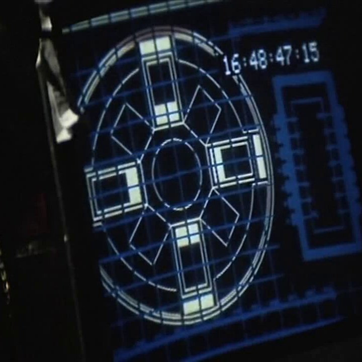
Ridley Scott's Film: Alien was produced by 20th Century Fox at Shepperton Studios in the UK. It required relevant information to be displayed on the 40 monitors of the space ship Nostromo's control deck including computer readouts, maps, space vistas and other videotaped graphics.
Tony was involved in a number of these animations using GRAM, FROLIC [7] (a FORTRAN-based system that was developed by Tony and Colin Emmett as an extension of ANTICS [8]) and sequences created at the Cambridge CAD Centre by Alan Sutcliffe.
Kate has already scanned about 300 pages of lineprinter listings related to Alien and only a subset of the GRAM code has been looked at in any detail.
Catherine Mason in her book A Computer in the Art Roome [6] states:
Alien was an early job for SSL involving Emmett, Lansdown, Pritchett, Sutcliffe, Wyvill, Mike Stapleton and others. Although Ridley Scott was a graduate of the RCA (where Mallen and others had connections), the commission came via Brunel through Mike Elstob.
The animation was carried out on a number of different machines, which demonstrates the overlap at the end of the decade in the use of mainframes and the (newer) micro-computer. These included the Atlas Lab's Prime 400 with FR80 plotter. They also used the Bugstore at the Cambridge Computer Aided Design Centre, which Emmett had previously used. Running this system was the software animation package FROLIC developed by Emmett.
Pritchett's initial graphic work ended up on the cutting room floor, but his second attempt, a few seconds of footage of the separation of the module of the spacecraft, was used and indeed appeared again, later, in Ridley Scott's motion picture Blade Runner (1982).
A simple example was part of the docking sequence, mentioned above, with the following scene on one of the main Nostromo monitors.
After looking though a great deal of GRAM code, we came across:
Some of these parts looked promising and we looked for appropriate GRAM code and, slightly modified to suit our version of GRAM, found:
:RING  146!5399     0  5379   470  5317   937  5215  1397 (
       )   5074  1846  4894  2282  4676  2699  4423  3097 (
       )   4136  3471  3818  3818  3471  4136  3097  4423 (
       )   2700  4676  2282  4894  1846  5074  1397  5215 (
       )    937  5317   470  5379     0  5399  -470  5379 (
       )   -937  5317 -1397  5216 -1846  5074 -2282  4894 (
       )  -2699  4676 -3097  4423 -3471  4136 -3818  3818 (
       )  -4136  3471 -4423  3097 -4676  2700 -4894  2282 (
       )  -5074  1846 -5215  1397 -5317   937 -5379   470 (
       )  -5399     0 -5379  -470 -5317  -937 -5216 -1397 (
       )  -5074 -1846 -4894 -2282 -4676 -2699 -4423 -3097 (
       )  -4136 -3471 -3818 -3818 -3471 -4136 -3097 -4423 (
       )  -2700 -4676 -2282 -4894 -1846 -5074 -1397 -5215 (
       )   -937 -5317  -470 -5379     0 -5399   470 -5379 (
       )    937 -5317  1397 -5216  1846 -5074  2282 -4894 (
       )   2699 -4676  3097 -4423  3471 -4136  3818 -3818 (
       )   4136 -3471  4423 -3097  4676 -2700  4894 -2282 (
       )   5074 -1846  5215 -1397  5317  -937  5379  -470 (
       )   5399     0 !5199     0  5180   453  5120   902 (
       )   5022  1345  4886  1778  4712  2197  4503  2599 (
       )   4259  2982  3983  3342  3676  3676  3342  3983 (
       )   2982  4259  2600  4503  2197  4712  1778  4886 (
       )   1345  5022   902  5120   453  5180     0  5199 (
       )   -453  5180  -902  5121 -1345  5022 -1778  4886 (
       )  -2197  4712 -2599  4503 -2982  4259 -3342  3983 (
       )  -3676  3676 -3983  3342 -4259  2982 -4503  2600 (
       )  -4712  2197 -4886  1778 -5022  1345 -5120   902 (
       )  -5180   453 -5199     0 -5180  -453 -5121  -902 (
       )  -5022 -1345 -4886 -1778 -4712 -2197 -4503 -2599 (
       )  -4259 -2982 -3983 -3342 -3676 -3676 -3342 -3983 (
       )  -2982 -4259 -2600 -4503 -2197 -4712 -1778 -4886 (
       )  -1345 -5022  -903 -5120  -453 -5180     0 -5199 (
       )    453 -5180   902 -5121  1345 -5022  1778 -4886 (
       )   2197 -4712  2599 -4503  2982 -4259  3342 -3983 (
       )   3676 -3676  3983 -3342  4259 -2982  4503 -2600 (
       )   4712 -2197  4886 -1778  5022 -1345  5120  -903 (
       )   5180  -453  5199     0
:PRB2 20!1800    800   800  1800  2000  3000  3000  2000  1800   800 (
     )  ! -800  1799 -1800   799 -3000  1999 -2000  2999  -800  1799 (
     )  !-1799  -800  -799 -1800 -1998 -3000 -2999 -2001 -1799  -800 (
     )  !  801 -1799  1800  -798  3001 -1997  2002 -2998   801 -1799
:RSEG 92!4100   1000  3948  1489  3739  1956  3475   2394  3159  2797 (
     )   2797   3159  2394  3475  1956  3739  1489   3948  1000  4100 (
     )   1000   5000  1527  4864  2038  4673  2525   4429  2983  4135 (
     )   3407   3793  3793  3407  4135  2983  4429   2525  4673  2038 (
     )   4864   1527  5000   999  4100  1000!-1000   4099 -1489  3947 (
     )  -1956   3738 -2394  3474 -2797  3158 -3159   2796 -3475  2393 (
     )  -3739   1955 -3948  1488 -4100   999 -5000    998 -4864  1525 (
     )  -4673   2036 -4429  2523 -4135  2981 -3793   3406 -3407  3792 (
     )  -2984   4134 -2526  4428 -2039  4672 -1528   4863 -1000  4999 (
     )  -1000 4099!-4099   -1001 -3947 -1490 -3738  -1957 -3473 -2395 (
     )  -3157  -2798 -2795 -3160 -2392 -3476 -1954  -3739 -1487 -3948 (
     )   -998  -4100  -997 -5000 -1524 -4864 -2035  -4673 -2522 -4430 (
     )  -2980  -4136 -3405 -3794 -3791 -3408 -4133  -2985 -4427 -2527 (
     )  -4672  -2040 -4863 -1529 -4999 -1001 -4099  -1001!1002  -4099 (
     )   1491  -3946  1958 -3737  2396 -3473  2799  -3156  3161 -2794 (
     )   3476  -2391  3740 -1953  3949 -1486  4100   -997  5000  -996 (
     )   4865  -1523  4674 -2034  4430 -2521  4137  -2979  3795 -3404 (
     )   3409  -3790  2986 -4132  2528 -4427  2041  -4671  1530 -4862 (
     )   1002  -4999  1002 -4099
:PRB1 50!-1800  -800 -1800   800  -800  1800   800  1800  1800   800 (
     )    1800  -800   800 -1800  -800 -1800 -1800  -800!1299      0 (
     )    1283   203  1236   401  1158   590  1051   764   919   919 (
     )     764  1051   590  1158   401  1236   203  1283     0  1299 (
     )    -203  1283  -401  1236  -590  1158  -764  1051  -919   919 (
     )   -1051   764 -1158   590 -1236   401 -1283   203 -1299     0 (
     )   -1283  -203 -1236  -401 -1158  -590 -1051  -764  -919  -919 (
     )    -764 -1051  -590 -1158  -401 -1236  -203 -1283     0 -1299 (
     )     203 -1283   401 -1236   590 -1158   764 -1051   919  -919 (
     )    1051  -764  1158  -590  1236  -401  1283  -203  1299     0
:NLOX 40! 1800 -800 1800 800 4400 800 4400 -800 1800 -800 (
) ! 2000  -600  2000   600  4200   600  4200  -600  2000   -600 (
) !  799  1800  -800  1799  -801  4399   798  4400   799   1800 (
) !  599  2000  -600  1999  -601  4199   598  4200   599   2000 (
) !-1800   799 -1799  -800 -4399  -802 -4400   797 -1800    799 (
) !-2000   599 -1999  -600 -4199  -602 -4200   597 -2000    599 (
) ! -798 -1800   801 -1799   803 -4399  -796 -4400  -798  -1800 (
) ! -598 -2000   601 -1999   603 -4199  -596 -4200  -598  -2000
:DOCKA 20!-800  -5000  800 -5000  800 -4600 -800 -4600 -800 -5000 (
) ! -5000   -800  -5000  800 -4600  800 -4600 -800 -5000 -800 (
) !  -800   4600    800 4600   800 5000  -800 5000  -800 4600 (
) !  4600   -800   4600  800  5000  800  5000 -800  4600 -800
:DOCKB1 20!-600 -2800 600 -2800 600 -2000 -600 -2000 -600 -2800 (
) ! -2800   -600 -2800    600 -2000   600 -2000  -600 -2800  -600 (
) !  -600   2800   600   2800   600  2000  -600  2000  -600  2800 (
) !  2000   -600  2000    600  2800   600  2800  -600  2000  -600
:DOCKB2 20!-600 -4200 600 -4200   600 -3400  -600 -3400 -600 -4200 (
) ! -4200   -600  -4200     600 -3400   600 -3400  -600 -4200 -600 (
) !  -600   4200    600    4200   600  3400  -600  3400  -600 4200 (
) !  3400   -600   3400     600  4200   600  4200  -600  3400 -600
:BURN[PICTURE DOCKS
:D1 1 1
:D2 100 100
AFTER 1
ANIM LIN 1
CH D1 100 100
CH D2 1 1
]
:DOCKS [
FIG RING
FIG PRB2
FIG PSEG
FIG PRB1
FIG NLOX
FIG DOCKA
PIC DOCK1
PIC DOCK2
  ]
:DOCK1[FIG DOCKB1
SCALE(D1)
   ]
:DOCK2[FIG DOCKB2
SCALE(D2)
   ]
VIEW BURN
1
2
3
T
STOP
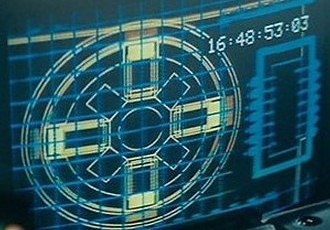
Clearly, in the film, some post processing has been done in converting the FR80 film output to the video played on the Nostromo monitor:
It was interesting to see that reuse is a concept in other areas besides computing. Here is a shot from the 1982 film Blade Runner.
A few more extensions to the GRAM system have been found in listings with dates later than the code in the working system we now have. In all cases the picture is incomplete, for example, FORTRAN code has been found for which the corresponding macro set is unknown and/or no examples of usage have been found. The subroutines USER, WOBBLE, SETWAV, WAVE and BURN are a case in point.
FORTRAN source code for these subroutines, plus code for SUBROUTINE USER, has been discovered in a listing dated 15 November 1978. There is a comment at the head of the source code: USER FOR TURBULENCE, STRESS AND DOCKING 29/6/78. From the form of the USER subroutine it is clear that these are three user-defined primitives. However although scripts have been found that use BURN, no scripts have yet been located that use WOBBLE, SETWAV and WAVE, though that is not to say that no such scripts exist. We will look briefly at BURN.
Subroutine BURN modifies the translation part of the transformation matrix at the current level in the tree by adding X, Y and Z increments to the current values of the translation components of the matrix. The increments are computed from the parameters supplied to BURN: an initial value (X,Y,Z), a starting value (VX,VY,VZ) and an increment (DX,DY,DZ). Each time the subroutine is called, (VX, VY, VZ) are incremented by (DX, DY, DZ) and the resulting values are added to (X, Y, Z). BURN can be invoked with all nine parameters or fewer. An example is:
PRIM BURN 107
:LAUNCH [ PICTURE SCENE
  :TURN 0
  ANIM LIN 10
  CH TURN 5
]
:SCENE [FIG PAD
  FIG TOWER
  ; arm disappears after frame 2
  IF(+FNO LT 3)[FIG ARM]
  PIC ROCKET
  ]
:ROCKET [
 FIG ROCKETSHAPE
 ROT(TURN)
 MOVE 0 -2000
 BURN 0 500 0
]
VIEW LAUNCH
1
2
3
4
5
6
7
8
9
10
T
STOP
Another feature of this example is the conditional expression:
IF(+FNO LT 3)[FIG ARM]
The effect is to display the arm linking the launch tower and the rocket if the requested frame number (in the variable FNO is less than 3. In other words, the arm is not displayed in frame 3 and subsequent frames. Conditional expressions are a key mechanism for controlling animations, usually wrapped up in higher level macros rather than written explicitly such as this example. A static view of the animation is shown below.
The effect is that the rocket appears to accelerate away from the launch pad over a period of 10 time steps, rotating slightly as it does so. (DX,DY,DZ) have been given values (0,500,0) and the other parameters will take initial default values of 0. BURN will be called each time a frame is requested. There are a number of problems with this, the main one being that this will not work with a more complex timeline structure, for example starting after some other animation has ended. BURN will be called irrespective of the timeline structure. This suggests that the primitive BURN was actually used in conjunction with a macro with the same name, but we have not as yet located script code to confirm this. As noted above, conditional expressions could be used explicitly to control invocations of the primitive or these could be within a macro body. That said, one script that has been found contains the sequence:
    ANIM LIN 75
    BURN 0 0 2
    THEN
    ANIM LIN 2 SEC
    BURN 0 0 0
    THEN
    ANIM LIN 5 SEC
    BURN 0 0 10
This would require BURN to be a macro, invoking the BURN primitive within the appropriate frame ranges, changing the (DX,DY,DZ) increments after 75 frames, a further 50 frames (2 sec) and a further 125 frames (5 sec).
Used in conjunction with a perspective projection, BURN can create the impression of an object accelerating into the distance. A basic example is shown below. The code is the same as the earlier rocket example, with the addition of the PERSP primitive to the ROCKET macro.
:ROCKET [
 FIG ROCKETSHAPE
 ROT(TURN)
 MOVE 0 -2000
 BURN 0 500 500
 PERSP 2400000
]
WOBBLE appears to modulate the fraction computed by LIN, but in the absence of examples of use, this will not be pursued here. For similar reasons, but also because the code appears to be incomplete, SETWAV and WAVE will not be discussed further either.
Various listings have been found, dated around July 1978, which contain coordinate definitions for a character font and various associated macro sets. The font is shown below.
The comments imply that this font was used to create some of the graffiti on the spaceship in Alien.
As Tony mentions in his letter to the BBC (Appendix 3):
GRAM has no specific type-face permanently set up in it. They are digitised as and when they are needed - normally 3 or 4 hours work on the digitiser at the Atlas Lab.
Earlier Terry came across font coordinates on tape TP14 that turned out to be mainly a set of digit characters in what looked like the Helvetica font presumably using a digitiser. Also Tony generated a "bank note" font with Stan Hayward that was used in a countdown sequence for an earlier project.
The GRAM system was in development/use from 1972 to 1978. In that period, there were significant changes in computers. Initially this was from early batch systems to ones that had simple interactive systems for job submission to a large batch main frame. At the same time, small computers became more powerful and it was feasible to do significant interactive work on such systems and by 1975 it was feasible to consider these small systems as multi-user interactive systems.
At the start of the period, generating multi-frame graphical output was primarily black and white line drawings on film using a microfilm recorder like the SC4020, designed to act as a fast lineprinter. By the end of the period, film recorders like the FR80 were capable of generating good quality colour filled-area scenes.
The GRAM system started life as a system for a small single-user computer able to define and produce simple graphics and animations relatively quickly. The initial environment constrained some of the decisions:
Tony wanted the system to be flexible, able to meet and execute new requirements quickly. The decision to base it on a macroprocessor and write it in FORTRAN was novel. There was knowledge of and involvement with the developments and use of Strachey's GPM at the University of London. Harwell had written a FORTRAN compiler in FORTRAN. This gave some confidence in the approach. Having X,Y coordinates and character pairs as the basic items that the macroprocessor manipulated was novel and less demanding on space than GPM. Allowing FORTRAN code to be used as primitive macros did allow flexibility in the way the system's usage could evolve.
Providing standard sets of macros for graphical input/output and animation definition was quite novel.
Early usage was simple drawings and animations while later it was possible to define and animate quite complex 3-D graphics.
There does not appear to be much use of GRAM after 1978. One reason might be the closure of the ICL 1906A in 1978 after the merger of the Atlas Computer Laboratory and Rutherford Laboratory. This removed Tony's main route to the FR80. Also, film was no longer the only way of generating graphics at both the BBC and the Open University.
We would like to thank Victoria Marshall at Chilton who made us aware of the possibilities, provided a home for online copies of the relevant manuals etc, and gave useful comments despite the lock down. Also Alex McGuinness who spent time looking at the computer monitors on Alien film clips trying to locate the work done on the FR80 that survived the cutting room.
1. A general purpose macrogenerator. C. Strachey, Computer Journal, Vol 8 No 3, 1965
2. FORTRAN IV: X3J3/90.4
3. Draft PhD Submission: Tony Pritchett
4. GRAM: Some Papers by Tony Pritchett
5. GRAM Manual, Chapters 1 to 6
6. A Computer in the Art Room by Catherine Mason, Quiller Press, 2008
7. FROLIC
8. ANTICS
9. GNU FORTRAN
12. BL120 Microfilm Recorder Technical Specification
13. ACL DMAC Manual
14. Chilton FR80
The FORTRAN code is a cut down version of the GRAM Nova FORTRAN code with a single input and output stream enhanced by additional debug output. The code for subroutines WOBBLE, SETWAV and WAVE is included, but has not been tested. As noted earlier, test cases for this code have not, so far, been found.
A second version of the code, with an enhanced SVG driver, has also been produced. The Nova FORTRAN code includes primitives to set three attributes for figures, colour, level and fade. The enhanced SVG driver ignores the level attribute, but translates colour to a class name and fade to an opacity value (percentage).
There are three changes from the standard code.
Using the rocket scene as an example, a simple case is:
FIG TOWER "GR"
The colour name "GR" is translated to the class name "GR" and the SVG code produced is:
<path class="GR" d="M -1000, -5500L -1000, -2000L -1200, -2000L -1200, -5500"/>
Colour names are restricted to one or two characters in the range A-Z or numbers in the usual range. Numbers are translated to a class name starting with underscore "_" character, followed by the number. This version of the GRAM program includes a CSS style file, svg_colour.css in the SVG and animated HTML generated. The user has the freedom to determine the content of this style file, which can include any CSS statements applicable to the SVG path element. For the example below, the contents are:
path.bdr  {stroke:blue;stroke-width:24;fill:none}
path      {stroke:green;stroke-width:12;fill:none}
path.RE {stroke:red}
path.BL {stroke:blue}
path.GR {stroke:green}
path.G {stroke:green; fill:green; opacity:20%}
path.OR {stroke:orange; fill:orange}
path._1 {stroke:orange; fill:orange}
Fade values are translated to a style attribute, for example:
<path class="_1" style="opacity:90%" d="M     0, -1500L   504, -1995
  L   530, -4995L   734, -5493L    30, -4999L  -665, -5505L  -469, -5004
  L  -495, -2004L     0, -1500"/>
draws the rocket filled in orange with opacity 90%.
The source code for a complete example (primitive and macro definitions omitted) is reproduced below. The opacity value of the rocket on each frame is computed by the FAD0 statement based on the current value of the frame number FNO. The complete input file, SVG file and HTML animation can be found in Appendix A2.
:ROCKETSHAPE 9!0 0 500 -500 500 -3500  700 -4000 0 -3500 (
  ) -700 -4000 -500 -3500 -500 -500 0 0
:TOWER 4! -1000 -5500 -1000 -2000 -1200 -2000 -1200 -5500
:ARM 4! -1000 -2700 -500 -2700 -500 -2750 -1000 -2750
:PAD 5!-2000 -6000 -2000 -5500 2000 -5500 2000 -6000 -2000 -6000
:OPAC 100
:LAUNCH [ PICTURE SCENE
  :TURN 0
  ANIM LIN 10
  CH TURN 5
]
:SCENE [FIG PAD "BL"
  FIG TOWER "G"
  ; arm disappears after frame 2
  IF(+FNO LT 3)[FIG ARM]
  PIC ROCKET
  ]
:ROCKET [
 FIG ROCKETSHAPE
 COLR 1
 FAD0 ((10-FNO)*10)
 ROT(TURN)
 MOVE 0 -2000
 BURN 0 500 0
]
If you have a FORTRAN compiler, it should be possible to run the following examples and get the appropriate output.
| Example | GRAM source | SVG output | SVG Animation |
|---|---|---|---|
| Animate triangle | anim_triangle.txt | anim_triangle.svg | anim_triangle.htm |
| Animate triangle (GRAM macros) | anim_triangle_macros.txt | anim_triangle_macros.svg | anim_triangle_macros.htm |
| Animated boat plus man and lighthouse | anim_boat.txt | anim_boat.svg | anim_boat.htm |
| Animated butterflies | anim_butterflies.txt | anim_butterflies.svg | anim_butterflies.htm |
| Alien Burn | alien.txt | alien.svg | anim_alien.htm |
| Rocket BURN | rocket_4.txt | rocket_4.svg | rocket_4.htm |
| Rocket BURN perspective | rocket_5.txt | rocket_5.svg | rocket_5.htm |
| Rocket BURN colour | rocket_6.txt | rocket_6.svg | rocket_6.htm |
Tony Pritchett
32 Winchester Rd.
London NW3 3NT
01-586 1329
John Richmond,Esq.
BBC Open University Productions
Alexandra Palace
London N22.
6 October 1976
Dear John,
As promised, I am writing to tell you about the computer animation system I have recently got working on the Nova computer in Technology faculty. The system is called GRAM (for GRAphic Macroprocessor). I will list some of its features:
It is interactive. One may sit down in front of a storage-tube v.d.u. and compose pictures using its graphic input facility like an "electronic drawing board". A script to animate the pictures may also be composed interactively, and putting the two together, one can view immediately any frame of the resulting sequences on the v.d.u. Unfortunately, it is not fast enough to display moving pictures.
Such a system provides a considerable saving in time over existing batch methods of doing computer animation. It is possible to compose a very simple animated sequence inside a few minutes, but I would normally expect to take considerably more time and trouble over even the simplest sequence for the O-U.
The GRAM system on the Nova at Milton Keynes cannot produce film directly, as it does not have the right hardware. This has to be done on the FR-80 microfilm recorder at the Atlas Lab, via tapes and the Atlas Lab's SMOG program.
The FR-80 can plot in colour direct1y on to colour film stock (negative or reversal, 16 or 35mm) without any registration problems.
There is also a system at the Atlas Lab which Colin Emmett and I have developed from the original ANTICS system which takes line images and scans them in to produce solid areas of colour ( and does hidden line removal at the same time). We haven't found a name for it yet, so we refer to it aa ANTICS MkII or SUPER ANTICS.
I am hoping for a turnround time of about a week for the simple moving graph type of sequence, using the Nova interactively and possibly handling more than one sequence at a time. However I would still have to allow much longer periods for the more sophisticated animations (one month or more).
The sequence of operations would be as follows:
This is very difficult to determine without any real-life operational experience with the system and without the following factors being known:
Having put forward these uncertainties, I am now going to stick my neck out and say that I would hope to do the simple moving graph stuff for under £100 per minute.
Colin and I have found that for the more sophisticated animation using Antics full colour shading, we have to quote £800 per minute minimum.
So there you have some ball-park extremes. Quoting "per minute" can also be misleading because the cost of computer animation is not nearly so dependent on footage than conventional animation, and more dependent on complexity. Thus a 30 sec sequence may cost £100, say, but extending it to 5 minutes doing the same thing will not put it up to £1000 but probably more like £300.
This is something you specially seemed concerned about. GRAM has no specific type-face permanently set up in it. They are digitised as and when they are needed - normally 3 or 4 hours work on the digitiser at the Atlas Lab.
Yours,
Tony
In a few of the scanned listings related to GRAM and Alien, it is not always clear whether the FORTRAN code and data refer to usage via GRAM or via other packages. There are listings that refer to other FORTRAN packages such as FROLIC, SPROGS, and ANTICS and also to the CAD Centre at Cambridge and a PRIME computer. Some data files clearly are aimed at GRAM whereas others may be input to another FORTRAN package, very likely to be FROLIC.
We think we have identified a crude font that might have been used to define graffiti on the space ship. Also, we believe the FORTRAN code for the image below may have been found:
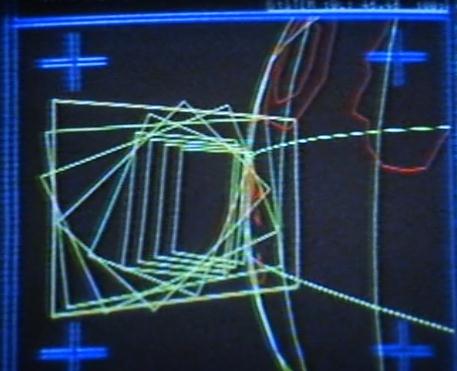
Some examples of comments etc on the relevant listings are:
C     BLOB's MESSAGE STUFF       (Blob is Brian Wyvill's nickname)
C     COLIN's SPHERE STUFF       (Colin Emmett)
C ROTATE BOTH PLANET AND BOXES BY HORIZON CONE ANGLE
C APPLY PERSPECTIVE TO BOTH PLANET AND BOXES
C LANDING SECTION, CIRCLE WITH DECREASING RADIUS
C SET 10 OR SO BOXES
C PLAN-ANIM FILES CONTAINS THE PLANET SPLIT INTO DAY AND NIGHT SIDES
 1    FORMAT("BUG STORE FILE NAME:")  (Bugstore was developed at the CAD Centre)
Terry Froggatt's home computer since 1978 has been an Elliott ARCH 9000 (the industrial version of Elliotts' commercial 903 or military 920B), with 16384 words of 18-bit core store, which had previously seen service at Mobil's Coryton oil refinery. In 2001, he interfaced its data port to the printer port of a conventional Personal Computer, enabling the PC to access the Elliott paper tape punch and reader as peripherals. Subsequently this was used to upload his extensive collection of paper tapes to the PC's filing system, and make them available via the Internet. From this point it was also possible to develop new software for the Elliott computer on the PC, without consuming quantities of paper tape.
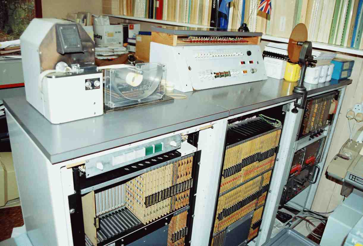
With this setup, it was straightforward to upload Tony's 75 paper tapes. Tape readers are not perfect, so each tape was uploaded at least twice and the uploads were compared. Most of Tony's tapes were 8-track, but there was one 5-track and one 7-track tape. When these tapes are read on an 8-track reader, one edge of the tape covers exactly half of a photocell, giving an unpredictable input, so it is necessary to mask out the unused tracks before the uploads are compared. The 7-track tape required a small change to the upload program, which previously had assumed tapes with a blank leader to be 8-track and tapes with a seemingly non-blank leader to be 5-track.
Some tapes presented the problem illustrated in TP04 below, where the tape started with punched characters rather than blank leader, and sometimes characters were missing.

With Kate's permission, Terry spliced a short length of blank leader onto these to read them. The characters were usually the name of the file, sometimes prefixed by the operating system command used to read or punch it. These names might usefully have appeared on a teleprinter listing at the time the tape was punched, but Terry imagines that once Tony had written the name onto the tape by hand, he deliberately tore the tape at this point to prevent the name being accidentally read later as part of the contents.
After checking and stripping parity when present, the 8-track tapes were all found to be in ASCII. The 5-track and 7-track tapes were converted to ASCII using these 5-code and 7-code definitions. Some new software was written to convert lists of coordinate pairs found in some of these text files into image files.
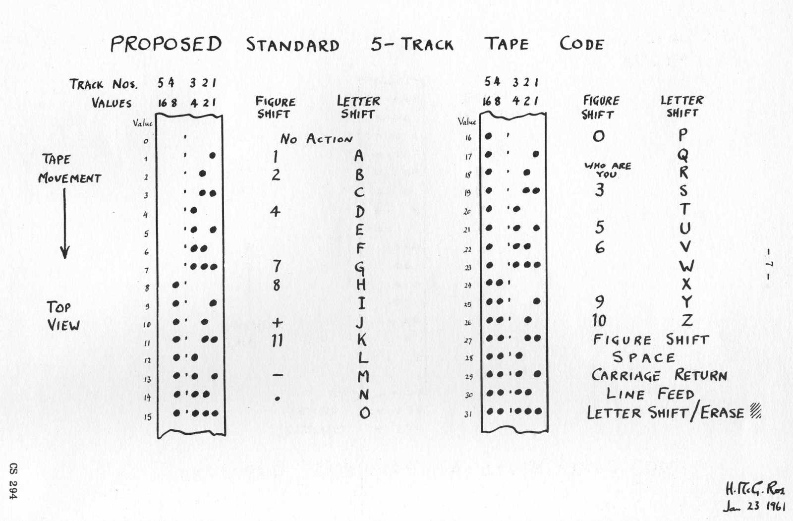
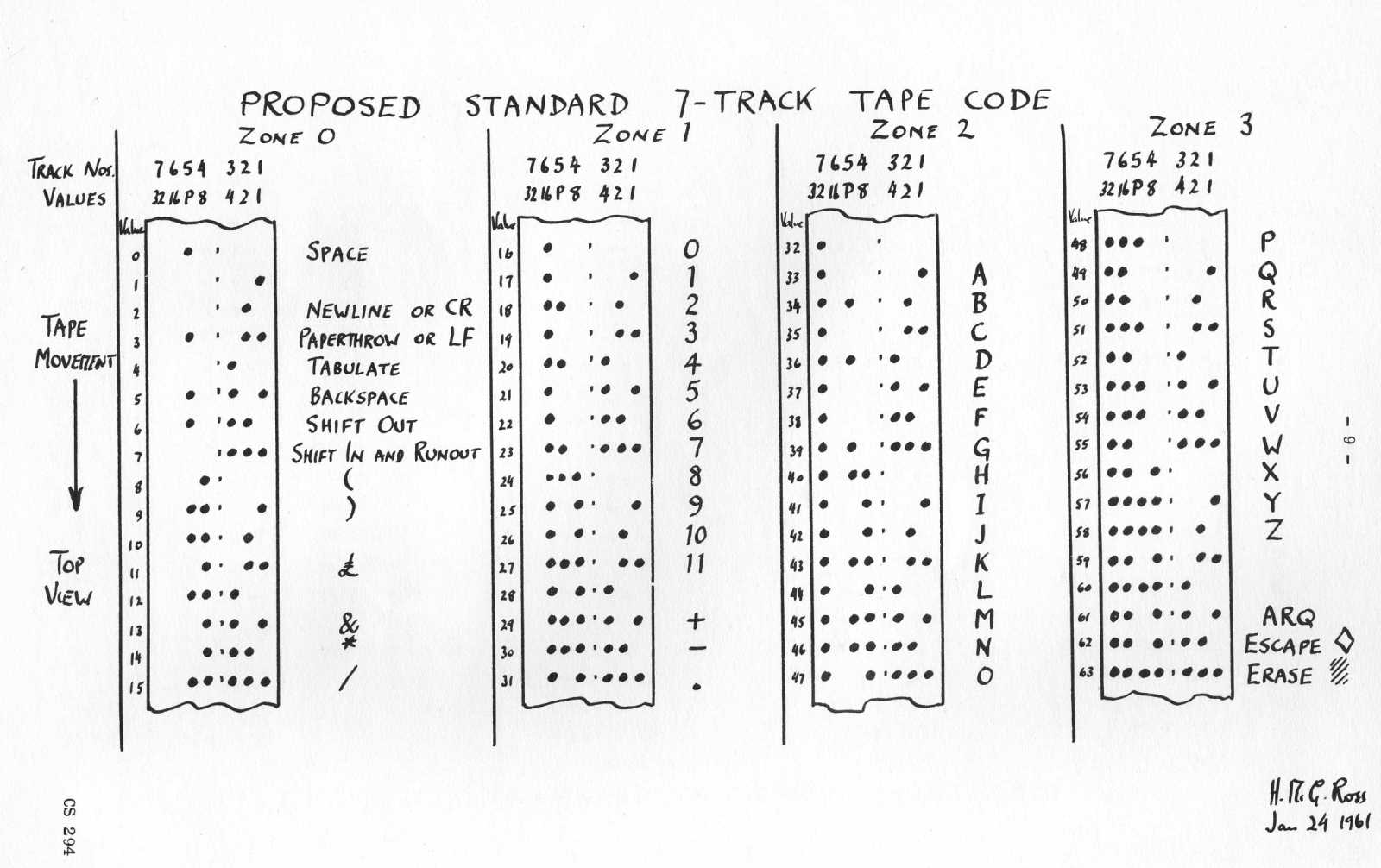