
This document provides a general review of all the facilities in the RAL GKS system. It is organized in a way which allows new users to start at the beginning and learn about successively more powerful facilities. All the routines in RAL GKS are mentioned and copious complete program examples are included.
This part is a User Guide to the RAL GKS package which runs on a large number of computer systems. The GKS implementation level is 2b.
GKS is a toolkit of facilities for the building of graphics programs in the area of two-dimensional line and raster graphics. It is implemented as a set of routines having a FORTRAN 77 interface with the programmer.
You are assumed to be familiar with FORTRAN 77 and with the machine and operating system that you are using. It is not assumed that you are familiar with computer graphics: from this view this guide is self contained.
For detailed specifications of the GKS routines and other reference material see the RAL GKS Reference Manual.
GKS is based on the principles of the ISO standard Graphical Kernel System but you do not have to be familiar with this standard.
Much of this guide consists of FORTRAN programs which illustrate the use of most of the routines in GKS, and the programs illustrate the combined use of several routines. In most cases the output of the program is also shown.
After reading this preface, you should read Chapter 1 which consists of a brief introduction to the GKS system in this context, and a section containing information on the running of any GKS program. The following chapters cover the facilities of GKS, starting with simple output and leading to more complex areas.
If you have experience of computer graphics you should then be able to proceed to particular chapters of immediate interest, but the reader without such experience should continue to read the chapters in sequence.
The text of this guide is divided into chapters in the normal way and each chapter is further divided into sections and sub-sections. The contents list and index, and cross-references in the text, all refer to chapter, section or sub-section numbers.
Figures and tables are numbered within chapters, as are the example programs and their output.
There is a long-standing need in computer graphics for international standards on a par with those evolved for computer programming languages, such as FORTRAN. Regional de facto standards do exist, for example GINO-F and GHOST in the UK and Calcomp-compatible packages in the USA. As changes in graphics devices occur, however, particularly in the rapidly growing area of raster graphics, these packages are becoming obsolete. The decision by the International Standards Organization (ISO) to define an international graphics standard was supported throughout the world and since 1978 there has been a thorough technical evaluation by graphics experts of many countries. The result is the Graphical Kernel System, published as an International Standard in 1985.
GKS is a standardized system of basic functions for graphical data processing in the area of two-dimensional line and raster graphics. The functions are defined independently of the device type, application and programming language. Implementations of GKS in any particular programming language consequently remain device and application independent. Graphical applications programs based on GKS thereby achieve device independence too.
GKS is a kernel system and so provides all the functions that a majority of applications want to use. Functions which are only suited to a particular application area may be provided in an application orientated layer on top of GKS; for example, graph plotting routines might appear in an application layer for data presentation. This means that the scope of GKS is different from some other graphics packages.
There are groups of routines in GKS which relate to:
GKS is defined independently of a programming language. In order to use GKS from FORTRAN 77, all the function names of GKS are mapped to FORTRAN subroutine names starting with G. The remaining letters are chosen by using a unique abbreviation of the single words of the function name; for instance ACTIVATE becomes AC, WORKSTATION becomes WK and so the FORTRAN subroutine name of ACTIVATE WORKSTATION is GACWK. For a list of all procedure names see the RAL GKS Reference Manual.
Names used internally in RAL GKS which may be visible outside GKS, for example during linking, start with GK (subroutine, function and COMMON block names). Therefore, when using GKS, no external names starting with GK should be chosen in order to avoid name conflict.
GKS has an error handling mechanism to report errors. If you require different information when an error occurs, you may provide your own error handling routine. You may even use the standard mechanism for most errors and your special routine for particular errors.
The GKS functions have parameters of several types. Most of these map directly onto equivalent data types in FORTRAN. One data type which does not, allows the specification of one of a number of alternatives and would be of enumerated type in Pascal. In FORTRAN, a name has been given to each alternative. These are in a parameter file (where they are assigned values in PARAMETER statements) which may be included in an application program. The statement to be inserted in the application program is machine-dependent and is described in Getting Started with RAL GKS1 and in Appendix B. A full list of these names is given in Appendix E. You must treat these names as reserved names if you include the parameter file in your program. Dummy argument names for enumerated values are implemented as INTEGER in FORTRAN 77. In this Guide these arguments start exclusively with the letter j .
All the examples in this User Guide are supplied with the RAL GKS software. To run an example, you need to compile it and link it with GKS. Instructions on how to compile, link, and run the examples are machine-dependent and are described in Getting Started with RAL GKS. In this Guide the examples use dummy argument names for workstation types, stream numbers and the GKS parameter file.
The machine-readable examples NODDY, and SHIP are device specific, but when you run most examples you will be prompted for the workstation type. The appearance of the output on your device may differ from the pictures in this Guide. Some examples may use facilities that are missing from your device (colour perhaps, or pattern fill). For such examples you will get informative error messages. A data file is supplied for input by example program CELLEX.
The box round the diagram indicates the boundary of the picture area. It is not output by the program as listed. The program that produced the output shown has an extra routine call to draw the box. The box shows where the output from the example program is placed on the screen.
Most of the example diagrams were drawn with a Calcomp 81 pen plotter driven by GKS running on a VAX 11/780.
Throughout this User Guide, the construct
GKS FUNCTION NAME (FORTRAN NAME)
is normally used when a routine is first introduced to you.
What do you need to do?
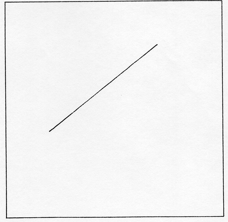
Example 1.1 shows one of the simplest GKS programs that it is possible to write. It draws the line shown in the diagram.
      PROGRAM NODDY
*                              GKS Example Program 1.1
                               The parameters for OPEN GKS and OPEN WORKSTATION
                               are for the VAX/VMS system; see Appendix B for
                               details of the values which are valid on each
                               system.
      REAL XA(2), YA(2)
      DATA  XA /0.2, 0.7/, YA /0.4, 0.8/
*
*                              Open GKS, errors to be noted on stream 6
      CALL GOPKS (6, -1)
*                              Open a Sigma 5684 workstation
      CALL GOPWK (1, 0, 106)
*                              Activate the workstation
      CALL GACWK (1)
*                              Draw a line
      CALL GPL   (2, XA, YA)
*                              Deactivate the workstation
      CALL GDAWK (l)
*                              Close the workstation
      CALL GCLWK (1)
*                              Close GKS
      CALL GCLKS
      END
First, you have to tell the system that you want to use GKS, by calling OPEN GKS (GOPKS).
Next you need to tell GKS which output device you want to use. GKS uses the term WORKSTATION to describe the device plus its software; the software compensates for any shortcomings in the device. OPEN WORKSTATION (GOPWK) is used to nominate the device. With the first parameter, you specify a number by which you will refer to the workstation in the rest of the program.
The next thing you need to do is activate the workstation. Once it is activated any output commands will cause output to appear on that device until you deactivate it. ACTIVATE WORKSTATION (GACWK) is used for this.
Later on when you have finished all the graphics that you require, you need to deactivate the workstation, close it down, and close GKS itself. Thus to tidy up before you finish executing the program call DEACTIVATE WORKSTATION (GDAWK), CLOSE WORKSTATION (GCLWK), both with the workstation identifier as parameter, and then CLOSE GKS (GCLKS). These control routines are fully discussed in Chapter 4.
Finally in this brief description of program 1.1 we examine the actual drawing of the line. The GKS philosophy is that most of the time users are not drawing a single line but whole sets of lines connected together. Consequently the only routine for drawing lines is POLYLINE (GPL). This draws a set of lines connecting the points XA(1),YA(1) to XA(2),YA(2) and XA(2),YA(2) to XA(3),YA(3) right up to XA(N-l),YA(N-1) to XA(N),YA(N).
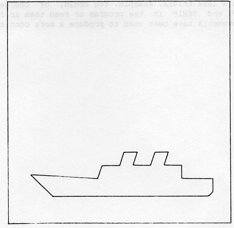
Program 1.2 shows a less trivial example. You could, of course, set the values of XSHIP and YSHIP in the program or read them in from a file. However, DATA statements have been used to produce a more concise example.
      PROGRAM SHIP
*                            GKS Example Program 1.2
                             The parameters for OPEN GKS and OPEN WORKSTATION
                             are for the VAX/VMS system; see Appendix B for
                             details of the values which are valid on each
                             system.
      REAL XSHIP(18), YSHIP(18)
      DATA XSHIP/0.20, 0.10, 0.40, 0.42, 0.50, 0.52, 0.58, 0.56,
     :           0.64, 0.66, 0.72, 0.70, 0.78, 0.78, 0.92, 0.92,
     :           0.90, 0.20/
      DATA YSHIP/0.12, 0.22, 0.20, 0.26, 0.26, 0.32, 0.32, 0.26,
     :           0.26, 0.32, 0.32, 0.26, 0,26, 0.20, 0.20, 0.14,
     :           0.12, 0,12/
*                            Open GKS, open Sigma, activate Sigma
      CALL GOPKS (6, -1)
      CALL GOPWK (1, 0, 106)
      Call GACWK (1)
*                            Draw the ship's outline
      CALL GPL (18, XSHIP, YSHIP)
*                            Deactivate Sigma, close it and close GKS
      CALL GDAWK (1)
      CALL GCLWK (1)
      CALL GCLKS
      END
The most obvious requirement for any graphics system is that it draws pictures. GKS has a richer set of functions for drawing than is common in comparable systems. The basic drawing actions are made available through two types of routine:
There are six GKS output primitive routines:
For POLYLINE, POLYMARKER, TEXT, FILL AREA and GDP you can control the appearance of the drawn objects. In GKS all output is produced according to the current value of some flags called OUTPUT ATTRIBUTES, so you change the representation by changing the attributes. There are many routines for doing this, because there are several attributes for each output primitive and the attributes for each primitive are separate.
There are obviously many different types of graphics device available, each with its own set of capabilities. Some may support a large number of colours, others only one. Some may have sufficient resolution for many different fonts to be distinguishable, others not.
As a user, you may want to get as close an approximation to a particular picture as possible. If the picture contains different colours but your device only supports one/ this may create a problem for you, since you may have been relying on the different colours to distinguish between different types of line (for example parish boundaries and footpaths).
The designers of GKS recognized this problem and provided two ways of using attributes:
The key idea about BUNDLED attributes is that a number of bundles are available and all those defined by the system are distinguishable on all workstations. As an example, consider the attributes that control POLYLINE output. As will be seen in section 2.3, there are three polyline attributes:
All of these are included in the polyline bundle. In GKS, five polyline bundles are predefined for all workstations. On a monochrome device, the predefined representation of these bundles is as follows:
| Bundle Index | Linetype | Linewidth Scale Factor | Colour Index |
|---|---|---|---|
| 1 | 1 | 1.0 | 1 |
| 2 | 2 | 1.0 | 1 |
| 3 | 3 | 1.0 | 1 |
| 4 | 4 | 1.0 | 1 |
| 5 | 5 | 1.0 | 1 |
so that linetype may be used to distinguish different bundles on a monochrome device. On colour displays, colour may be used instead:
| Bundle Index | Linetype | Linewidth Scale Factor | Colour Index |
|---|---|---|---|
| 1 | 1 | 1.0 | 1 |
| 2 | 1 | 1.0 | 2 |
| 3 | 1 | 1.0 | 3 |
| 4 | 1 | 1.0 | 4 |
| 5 | 1 | 1.0 | 5 |
You may set the representation of a bundle and this allows you to use bundles in another way. They can be useful as a shorthand notation. The most obvious example is in map drawing, where it would be natural to set up bundles for all the conventional line representations, such as
footpath     dotted, thin,  red
bridleway    dashed, thin,  red
path         dashed, thin,  black
river        solid,  thin,  blue
railway      solid,  thick, black
Individual attributes should be used when the closest picture is required rather than a picture in which elements are necessarily distinguishable. Different workstations may not be able to do anything about some attribute changes but the available attributes will be matched as closely as possible.
For example, if you need to draw with ten different linetypes on one graph and ten were available on the plotter you were using for the final output, you could select linetypes 1 to 10 in succession. This would work on the plotter and would be simpler than defining and then using ten bundles. However, if you previewed the output on a device with fewer linetypes, the remaining ones would all appear solid.
You have to indicate whether you want to use bundled or individual attributes. By default, bundled attributes are used. This may be changed, for each attribute separately, by the routine SET ASPECT SOURCE FLAGS (GSASF): this is described fully in section 2.9.
GKS has a powerful system for dealing with colour as an attribute and as an element of the CELL ARRAY primitive. All colours are specified in GKS by means of indices into a COLOUR TABLE; there is a separate colour table for each workstation. As a result, in the following sections, a number of references to COLOUR INDICES are made. There is a complete explanation of the colour system in GKS in section 2.10.
In GKS all line drawing is done by routine POLYLINE.
GPL (npoint, xa, ya)
This takes a list of points and connects the first to the second, the second to the third and so on. The number of points is given by npoint and the X and Y coordinates of each point are in the REAL arrays xa and ya. The operation of POLYLINE may be seen in example 2.1.
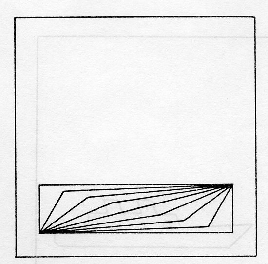
GKS will not modify the parameters passed to POLYLINE, so the same arrays can be used over and over again as in example 2.2 where a set of related polylines are drawn.
      PROGRAM POLY1
*                                 GKS Example Program 2.1
*                                 Data for Ship's Outline
      INTEGER NSHIP
      PARAMETER (NSHIP = 18)
      REAL XSHIP(NSHIP), YSHIP(NSHIP)
      DATA XSHIP/0.20,0.10,0.40,0.42,0.50,0.52,0.58,0.56,0.64,
     :          0.66,0.72,0.70,0.78,0.78,0.92,0.92,0.90,0.20/
     :     YSHIP/0.12,0.22,0.20,0.26,0.26,0.32,0.32,0.26,0.26,
     :           0.32,0.32,0.26,0.26,0.20,0.20,0.14,0.12,0.12/
*                                OPEN GKS, OPEN and ACTIVATE WORKSTATION. The
*                                parameters for OPEN GKS and OPEN WORKSTATION
*                                are system- and device- dependent; see Appendix B
*                                for details of the values which are valid on each
*                                system.
      CALL GOPKS (kerrfl, -1)
      CALL GOPWK (1 , kconid, kwtype)
      CALL GACWK (1)
*                                End of standard opening sequence
*----------------------------------------------------------------------------------
      CALL GPL (NSHIP , XSHIP , YSHIP)
*----------------------------------------------------------------------------------
*                               Deactivate and close workstation, close GKS
      CALL GDAWK (1)
      CALL GCLWK (1)
      CALL GCLKS
      END
      PROGRAM POLY2
*                                 GKS Example Program 2.2
      REAL XA(3), YA(3), XDIFF, YDIFF
      DATA XA/0.1,0.0,0.9/ YA/0.1,0.325,0.3/
      DATA XDIFF/0.1/ YDIFF/0.025/
*                                OPEN GKS, OPEN and ACTIVATE WORKSTATION. The
*                                parameters for OPEN GKS and OPEN WORKSTATION
*                                are system- and device- dependent; see Appendix B
*                                for details of the values which are valid on each
*                                system.
      CALL GOPKS (kerrfl, -1)
      CALL GOPWK (1 , kconid, kwtype)
      CALL GACWK (1)
*                                End of standard opening sequence
*----------------------------------------------------------------------------------
      DO 10 J=1,9
      XA(2) = XA(2) + XDIFF
      YA(2) = YA(2) - YDIFF
      CALL GPL (3 , XA , YA)
   10 CONTINUE
*----------------------------------------------------------------------------------
*                               Deactivate and close workstation, close GKS
      CALL GDAWK (1)
      CALL GCLWK (1)
      CALL GCLKS
      END
POLYLINE output is controlled by three attributes, all of which are included in the polyline bundle. The following routines may be used to change the polyline index, bundle representations and individual attributes. The first, SET POLYLINE INDEX, selects a particular bundle of polyline attributes:
GSPLI (kpli)
The kpli must be positive and may refer to a predefined bundle or one that you have defined by SET POLYLINE REPRESENTATION:
GSPLR (kwkid, kpli, lntype, width, kplcol)
This creates or changes the representation of a polyline bundle for a particular workstation. The workstation with identifier kwkid has its polyline bundle with index kpli set to a representation with linetype lntype, linewidth scale factor width and colour index kplcol. For some workstations, this will cause all output created with this index to be modified (see Section 2.11, Implicit Regeneration).
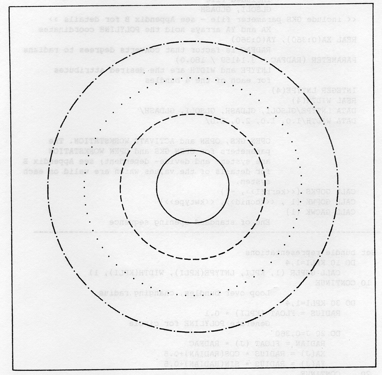
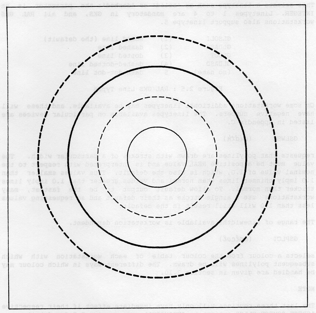
In example 2.3, a nested group of circles are drawn, each with a different POLYLINE INDEX, showing the different bundles. If you want the representations of the bundles to be as shown in figure 2.4 you will have to set the representations yourself, as is shown in example 2.4.
| Bundle Index | Linetype | Linewidth Scale Factor | Colour Index |
|---|---|---|---|
| 1 | 1 | 1.0 | 1 |
| 2 | 2 | 1.0 | 1 |
| 3 | 1 | 2.0 | 1 |
| 4 | 1 | 2.0 | 1 |
      PROGRAM CIRCLE
*                                 GKS Example Program 2.3
*                                 XA and YA arrays hold the polyline coordinates
      REAL XA(0:360), YA(0:360)
*                                 RADFAC is a factor that converts degrees to radians
      REAL RADFAC
      PARAMETER (RADFAC = 3.14.159 / 180.0)
      DATA XDIFF/0.1/ YDIFF/0.025/
*                                OPEN GKS, OPEN and ACTIVATE WORKSTATION. The
*                                parameters for OPEN GKS and OPEN WORKSTATION
*                                are system- and device- dependent; see Appendix B
*                                for details of the values which are valid on each
*                                system.
      CALL GOPKS (kerrfl, -1)
      CALL GOPWK (1 , kconid, kwtype)
      CALL GACWK (1)
*                                End of standard opening sequence
*----------------------------------------------------------------------------------
*                                Loop over bundles, changing radius
      DO 20 KPLI=1,4
      RADIUS = FLOAT (KPLI) * 0.1
*                                Generate POLYLINE for circle
*                                (note that (XA(0) ,YA(0)) = (XA(360) ,YA(360)))
      DO 10 J=0,360
      RADIAN = FLOAT (J) * RADFAC
      XA(J) = RADIUS * COS(RADIAN)+0.5
      YA(J) = RADIUS * SIN(RADIAN)+0.5
   10 CONTINUE
*                                Set POLYLINE bundle index
      CALL GSPLI (KPLI)
*                                Draw the circle
      CALL GPL   (361 , XA , YA)
   20 CONTINUE
*----------------------------------------------------------------------------------
*                               Deactivate and close workstation, close GKS
      CALL GDAWK (1)
      CALL GCLWK (1)
      CALL GCLKS
      END
      PROGRAM CIRCLE
*                                 GKS Example Program 2.4
*                                 The following variable(s) are defined in the
*                                 included file
*                                 GLSOLI, GLDASH
*                                 include GKS parameter file - see Appendix B for details
*                                 XA and YA arrays hold the POLYLINE coordinates
      REAL XA(0:360), YA(0:360)
*                                 RADFAC is a factor that converts degrees to radians
      PARAMETER (RADFAC = 3.14.159 / 180.0)
*                                 LNTYPE and WIDTH are the desired attributes
*                                 for each of the 4 bundles
      INTEGER LNTYPE(4)
      REAL WIDTH(4)
      DATA LNTYPE/GLSOLI, GLDASH, GLSOLI, GLDASH/
      DATA WIDTH/1.0, 1.0, 2.0, 2.0/
*                                OPEN GKS, OPEN and ACTIVATE WORKSTATION. The
*                                parameters for OPEN GKS and OPEN WORKSTATION
*                                are system- and device- dependent; see Appendix B
*                                for details of the values which are valid on each
*                                system.
      CALL GOPKS (kerrfl, -1)
      CALL GOPWK (1 , kconid>, kwtype)
      CALL GACWK (1)
*                                End of standard opening sequence
*----------------------------------------------------------------------------------
*                                Set bundle representations
      DO 10 KPLI=1,4
      CALL GSPLR (1, KPLI, LNTYPE(KPLI), WIDTH(KPLI), 1)
   10 CONTINUE
*                                Loop over bundles, changing radius
      DO 30 KPLI=1,4
      RADIUS = FLOAT (KPLI) * 0.1
*                                Generate POLYLINE for circle
      DO 20 J=0,360
          RADIAN = FLOAT (J) * RADFAC
          XA(J) = RADIUS * COS(RADIAN)+0.5
          YA(J) = RADIUS * SIN(RADIAN)+0.5
  20  CONTINUE
*                                Set POLYLINE bundle index
      CALL GSPLI (KPLI)
*                                Draw the circle
      CALL GPL   (361, XA, YA)
   30 CONTINUE
*----------------------------------------------------------------------------------
*                               Deactivate and close workstation, close GKS
      CALL GDAWK (1)
      CALL GCLWK (1)
      CALL GCLKS
      END
If you are using INDIVIDUAL attributes, three routines provide access to these: SET LINETYPE, SET LINEWIDTH SCALE FACTOR and SET POLYLINE COLOUR INDEX:
GSLN (lntype)
This selects a linetype such as solid or dashed: the parameter is an INTEGER. Linetypes 1 to 4 are mandatory in GKS, and all RAL GKS workstations also support linetype 5.
      GLSOLI    (1) solid line (the default)
      GLDASH    (2) dashed line
      GLDOT     (3) dotted line
      GLDASD    (4) dashed-dotted line
      (no name)  5  dash-dot-dot line
On some workstations additional linetypes may be available, and these will have negative numbers. The linetypes available on particular devices are listed in Appendix C.
GSLWSC (width)
requests that polylines are drawn with strokes of a particular width. The value must be a positive REAL value and is interpreted with respect to the nominal value of 1.0, which is also the default. Thus values smaller than 1.0 imply thinner lines than normal and values greater than 1.0 imply lines thicker than normal. To allow default output to be the fastest, many workstations use a single stroke as their default and so requesting values less than 1.0 will still result in the default.
The range of linewidths available is workstation dependent.
GSPLCI (kplcol)
selects a colour from the colour table of each workstation with which subsequent polylines will be drawn. The different ways in which colour may be handled are given in section 2.10.
The last three routines will only have immediate effect if their respective ASPECT SOURCE FLAGS are set to INDIVIDUAL: see section 2.9 for details.
Example 2.5 shows how individual attributes are used. The output is the same as example 2.4.
      PROGRAM CIRIND
*                                 GKS Example Program 2.5
*                                 The following variable(s) are defined in the
*                                 included file
*                                 GINDV, GLSOLI, GLDASH
*                                 include GKS parameter file - see Appendix B for details
*                                 Set up parameters with names for the ASFs
      INTEGER    GALN,      GALWSC,    GAPLCI,   GAMK,     GAMKSC
      PARAMETER (GALN=1,    GALWSC=2,  GAPLCI=3, GAMK=4,   GAMKSC=5)
      INTEGER    GAPMCI,    GATXFP,    GACHXP,   GACHSP,   GATXCI
      PARAMETER (GAPMCI=6,  GATXFP=7,  GACHXP=8, GACHSP=9, GATXCI=10)
      INTEGER    GAFAIS,    GAFASI,    GAFACI
      PARAMETER (GAFAIS=11, GAFASI=12, GAFACI=13)
*                                 JASF is an array that holds the ASFS
      INTEGER JASF(13)
*                                 XA and YA arrays hold the POLYLINE coordinates
      REAL XA(0:360), YA(0:360)
*                                 RADFAC is a factor that converts degrees to radians
      PARAMETER (RADFAC = 3.14.159 / 180.0)
*                                 LNTYPE and WIDTH are the desired attributes
*                                 for each of the 4 bundles
      INTEGER LNTYPE(4)
      REAL WIDTH(4)
      DATA LNTYPE/GLSOLI, GLDASH, GLSOLI, GLDASH/
      DATA WIDTH/1.0, 1.0, 2.0, 2.0/
*                                OPEN GKS, OPEN and ACTIVATE WORKSTATION. The
*                                parameters for OPEN GKS and OPEN WORKSTATION
*                                are system- and device- dependent; see Appendix B
*                                for details of the values which are valid on each
*                                system.
      CALL GOPKS (kerrfl, -1)
      CALL GOPWK (1 , kconid, kwtype)
      CALL GACWK (1)
*                                End of standard opening sequence
*----------------------------------------------------------------------------------
*                                Inquire current ASFs and set LINETYPE and
*                                LINEWIDTH SCALE FACTOR to be INDIVIDUAL
      CALL GQASF (KERROR, JASF)
      JASF(GALN) = GINDIV
      JASF(GALWSC) = GINDIV
      CALL GSASF (JASF)
*                                Loop over linetypes and linewidths, changing radius
      DO 20 KPLI=1,4
       RADIUS = FLOAT (KPLI) * 0.1
*                                Generate POLYLINE for circle
       DO 10 J=0,360
        RADIAN = FLOAT (J) * RADFAC
        XA(J) = RADIUS * COS(RADIAN}+0.5
        YA(J) = RADIUS * SIN(RADIAN)+Q.5
 10    CONTINUE
*                                Set linetype and linewidth
      CALL GSLN   (LNTYPE(KPLI))
      CALL GSLWSC (WIDTH(KPLI))
*                                Draw the circle
      CALL GPL {361 , XA , YA)
   20 CONTINUE
*----------------------------------------------------------------------------------
*                               Deactivate and close workstation, close GKS
      CALL GDAWK (1)
      CALL GCLWK (1)
      CALL GCLKS
      END
You have seen that POLYLINE provides the most obvious form of output, that of straight lines. Another useful facility is that of placing markers (symbols) at. specific positions. For this, you use POLYMARKER.
GPM (npoint, xa, ya)
POLYMARKER will place the currently selected marker at each of the positions given in the xa, ya. arrays. The number of points is given by npoint.
The attributes that describe the marker are its TYPE (for instance an asterisk, a circle or a dot), its relative size (specified as a MARKER SIZE SCALE FACTOR) and its colour, specified as usual by a COLOUR INDEX. All these attributes are included in the POLYMARKER BUNDLE. The two routines for handling POLYMARKER BUNDLES are SET POLYMARKER INDEX and SET POLYMARKER REPRESENTATION:
GSPMI (kpmi)
After this has been called, subsequent markers are produced according to the representation of bundle kpmi. If you want to change the representation, you call
GSPMR (kwkid, kpmi, mktype, sizemk, kpmcol)
which changes the representation of polymarker bundle kpmi on workstation kwkid; mktype is the marker type, sizemk is the marker size scale factor and kpmcol the colour index. For some workstations, this will cause all output created with this index to be modified (see Section 2.11, Implicit Regeneration).
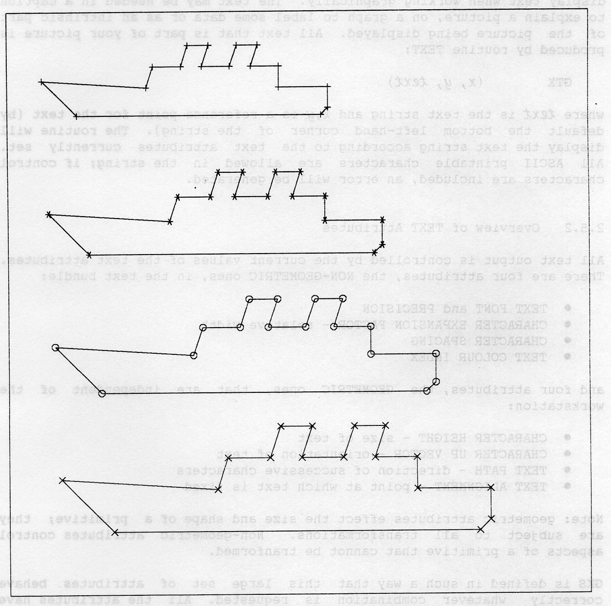
All workstations support marker types 1 to 5 and must display them as in figure 2.6.
GPOINT      (1)     .      dot
GPLUS       (2)     +      vertical cross
GAST        (3)     *      asterisk
GOMARK      (4)     o      circle
GXMARK      (5)     x      diagonal cross
Marker type 1 is the smallest displayable dot and is unaffected by the marker size scale factor. It is useful when drawing scatter plots and such forms of output. However, if you want a large array of dots (of different colour or intensity) do not think of using lots of dots with POLYMARKER: GKS has a routine (CELL ARRAY, see section 2.7) for producing images and it will, in general, be vastly faster and simpler to use.
Each of the polymarker attributes may be set individually, using routines SET MARKERTYPE, SET MARKER SIZE SCALE FACTOR and SET POLYMARKER COLOUR INDEX:
GSMK       (mktype,)
GSMKSC     (sizemk)
GSPMCI     (kpmcol)
As before, these routines will only be effective if the corresponding ASPECT SOURCE FLAGS are set to INDIVIDUAL, which is not the default (see section 2.9). The default individual marker type is the asterisk.
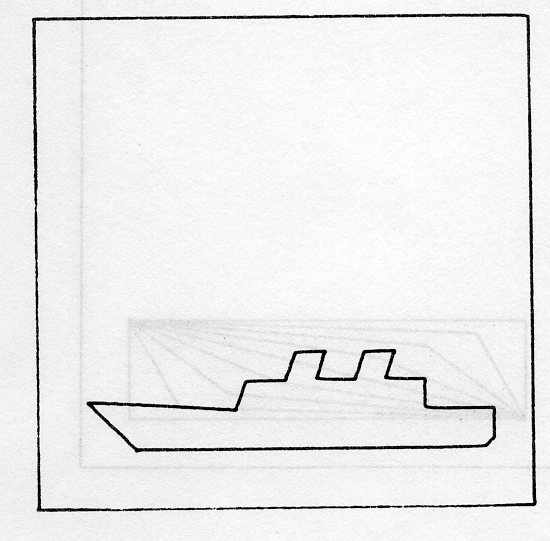
Example 2.6 shows how POLYMARKER is used and demonstrates how it can be combined with POLYLINE to produce easily distinguishable output in graphical applications.
      PROGRAM Marker
*                                 GKS Example Program 2.6
*                                 Data for Ship's Outline
      INTEGER NSHIP
      PARAMETER (NSHIP = 18)
      REAL XSHIP(NSHIP), YSHIP(NSHIP)
      DATA XSHIP/0.20,0.10,0.40,0.42,0.50,0.52,0.58,0.56,0.64,
     :          0.66,0.72,0.70,0.78,0.78,0.92,0.92,0.90,0.20/
     :     YSHIP/0.12,0.22,0.20,0.26,0.26,0.32,0.32,0.26,0.26,
     :           0.32,0.32,0.26,0.26,0.20,0.20,0.14,0.12,0.12/
*                                OPEN GKS, OPEN and ACTIVATE WORKSTATION. The
*                                parameters for OPEN GKS and OPEN WORKSTATION
*                                are system- and device- dependent; see Appendix B
*                                for details of the values which are valid on each
*                                system.
      CALL GOPKS (kerrfl, -1)
      CALL GOPWK (1 , kconid, kwtype)
      CALL GACWK (1)
*                                End of standard opening sequence
*----------------------------------------------------------------------------------
*                                Set scaling factor for ship's outline
      DO 20 KPMI=2,5
      FACTOR = 0.5 + FLOAT (KPMI-l) * 0.1
      DO 10 J=1,NSHIP
       XTEMP(J) = XSHIP(J) * FACTOR
       YTEMP(J) = YSHIP(J) * FACTOR+1.0-FLOAT(KPMI-1)*0.25
 10   CONTINUE
*                                Set POLYMARKER bundle index
      CALL GSPMI (KPMI)
*                                Draw the outline as solid POLYLINE
      CALL GPL (NSHIP, XTEMP, YTEMP)
*                                Mark, each vertex with a marker
*                                No need to do last point, which is a
*                                duplicate of the first in this case
      CALL GPM (NSHIP-1, XTEMP, YTEMP)
   20 CONTINUE
*----------------------------------------------------------------------------------
*                               Deactivate and close workstation, close GKS
      CALL GDAWK (1)
      CALL GCLWK (1)
      CALL GCLKS
      END
In addition to lines and markers, there is an obvious need to be able to display text when working graphically. The text may be needed in a caption to explain a picture, on a graph to label some data or as an intrinsic part of the picture being displayed. All text that is part of your picture is produced by routine TEXT:
GTX (x, y, text)
where text is the text string and x, y is a reference point for the text (by default the bottom left-hand corner of the string). The routine will display the text string according to the text attributes currently set. All ASCII printable characters are allowed in the string; if control characters are included, an error will be generated.
All text output is controlled by the current values of the text attributes. There are four attributes, the NON-GEOMETRIC ones, in the text bundle:
and four attributes, the GEOMETRIC ones, that are independent of the workstation:
Note: geometric attributes effect the size and shape of a primitive; they are subject to all transformations. Non-geometric attributes control aspects of a primitive that cannot be transformed.
GKS is defined in such a way that this large set of attributes behave correctly whatever combination is requested. All the attributes have sensible default values to enable you to produce text without having to specify all the attributes every time.
Figure 2.7 demonstrates the use of various text attributes.
Several FONTS are available and each may only be available to a particular PRECISION. The setting routine is given in Section 2.5.6. There are three precisions defined; in order of ascending fidelity they are:
Fonts are identified by a font number as in the following table.
Number  Contents of Font
 1   Standard hardware text (device dependent)
-101 Roman,   Medium,     Sans Serif
-102 Roman,   Bold,       Sans Serif
-103 Greek,   Medium,     Sans Serif
-104 Roman,   Medium,     Seriffed
-105 Roman,   Italic,     Seriffed
-106 Roman,   Bold,       Seriffed
-107 Roman,   Bold Italic, Seriffed
-108 Reserved for future use
-109 Reserved for future use
-110 Greek,   Medium,     Seriffed
-111 Reserved for future use
-112 Reserved for future use
-113 Reserved for future use
-114 Reserved for future use
-115 Mathematical
(Serifs are the little feet that normal printed characters have; sans serif means the characters have no serifs.)
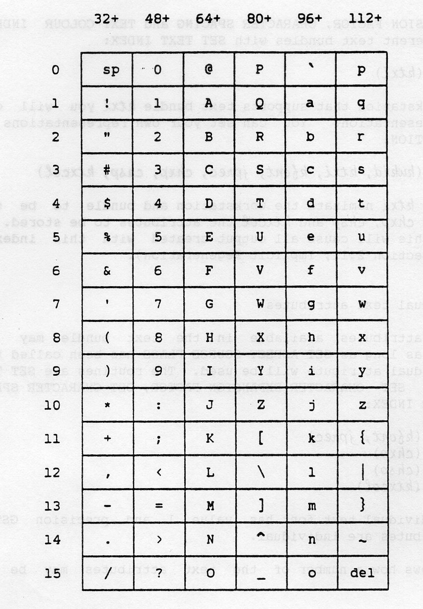
All the fonts are displayed in Appendix D; the standard character set is the one shown in the following figure. The graphic character is shown against its position in the ASCII table for reference.
If your workstation has colour capability, you can change the colour of the text:
GSTXCI (ktxcol)
The text is then produced in the colour whose index in the device colour table is ktxcol.
The text bundle consists of the attributes TEXT FONT AND PRECISION, CHARACTER EXPANSION FACTOR, CHARACTER SPACING and TEXT COLOUR INDEX. You can select different text bundles with SET TEXT INDEX:
GSTXI (ktxi)
and on each workstation that supports text bundle ktxi you will obtain a new text representation. You can set your own representations with SET TEXT REPRESENTATION:
GSTXR (kwkid, ktxi, kfont, jprec, chxp, chsp, ktxcol)
where kwkid and ktxi nominate the workstation and bundle to be set, and kfont, jprec, chxp, chsp and ktxcol the attributes to be stored. For some workstations, this will cause all output created with this index to be modified (see Section 2.11, Implicit Regeneration).
Each of the attributes available in the text bundle may be set individually, as long as SET ASPECT SOURCE FLAGS has been called to ensure that the individual attribute will be used. The routines are SET TEXT FONT AND PRECISION, SET CHARACTER EXPANSION FACTOR, SET CHARACTER SPACING and SET TEXT COLOUR INDEX:
GSTXFP    (kfont, jprec)
GSCHXP    (chxp)
GSCHSP    (chsp)
GSTXCI    (ktxcol)
The default individual text font has value 1 and precision GSTRP. All geometric attributes are individual.
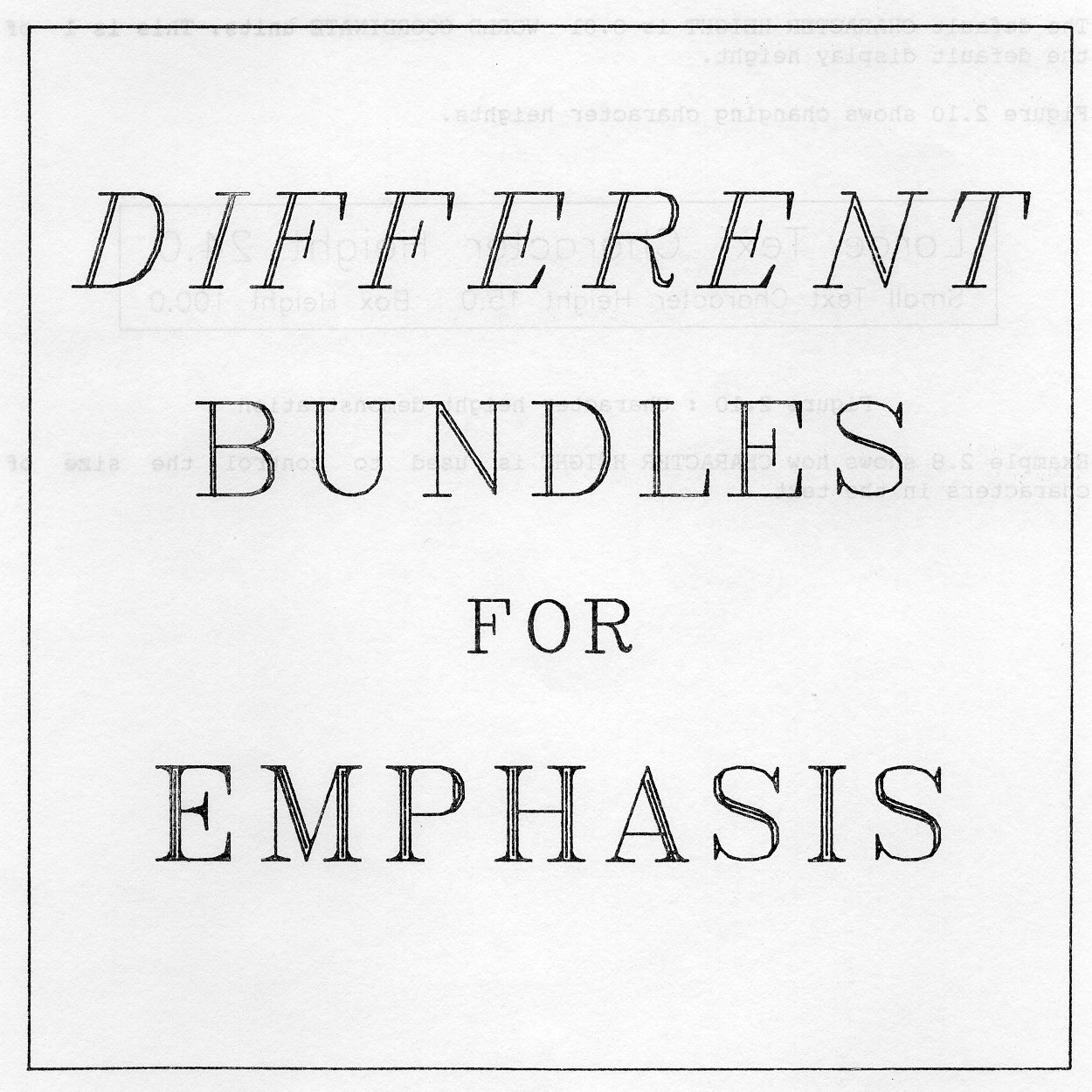
Example 2.7 shows how a number of the text attributes may be used in bundles.
      PROGRAM TESTEX
*                                 GKS Example Program 2.7
*                                 The following variable(s) are defined in the
*                                 included file
*                                 GINDIV, GACHXP, GACHSP, GSTRKP, GACENT, GABASE
*                                 include GKS parameter file - see Appendix B for details
*                                 Set up parameters with names for the ASFs
      INTEGER    GALN,      GALWSC,    GAPLCI,   GAMK,     GAMKSC
      PARAMETER (GALN=1,    GALWSC=2,  GAPLCI=3, GAMK=4,   GAMKSC=5)
      INTEGER    GAPMCI,    GATXFP,    GACHXP,   GACHSP,   GATXCI
      PARAMETER (GAPMCI=6,  GATXFP^7,  GACHXP=8, GACHSP=9, GATXCI=10)
      INTEGER    GAFAIS,    GAFASI,    GAFACI
      PARAMETER (GAFAIS=11, GAFASI=12, GAFACI=13)
*                                 JASF is an array that holds the ASFS
      INTEGER JASF(13)
*                                OPEN GKS, OPEN and ACTIVATE WORKSTATION. The
*                                parameters for OPEN GKS and OPEN WORKSTATION
*                                are system- and device- dependent; see Appendix B
*                                for details of the values which are valid on each
*                                system.
      CALL GOPKS (kerrfl, -1)
      CALL GOPWK (1 , kconid, kwtype)
      CALL GACWK (1)
*                                End of standard opening sequence
*----------------------------------------------------------------------------------
*                                Set ASPECT SOURCE FLAG for CHARACTER EXPANSION
*                                FACTOR and CHARACTER SPACING to INDIVIDUAL
      CALL GQASF (KERROR, JASF)
      JASF(GACHXP) = GINDIV
      JASF(GACHSP) = GINDIV
      CALL GSASF (JASF)
*                                Set bundle representations
      CALL GSTXR (1, 1, -104, GSTRKP, 1.0, 0.0, 1)
      CALL GSTXR (1, 2, -105, GSTRKP, 1.0, 0.0, l)
      CALL GSTXR (1, 3, -106, GSTRKP, 1.0, 0.0, l)
*                                Increase character spacing for all strings
      CALL GSCHSP (0.1)
*                                Set alignment to centre strings
      CALL GSTXAL (GACENT, GABASE)
*                                Set larger characters
      CALL GSCHH (0.09)
*                                Draw text with different bundle indices
      CALL GSTXI (2)
      CALL GTX (0.5, 0.75, 'DIFFERENT')
      CALL GSTXI (1)
      CALL GTX (0.5, 0.55, 'BUNDLES')
*                                Set smaller characters
      CALL GSCHH (0.05)
      CALL GTX (0.5, 0.4, 'FOR')
*                                Restore larger characters
      CALL GSCHH (0.09)
      CALL GSTXI (3)
      CALL GTX (0.5, 0.2, 'EMPHASIS')
*----------------------------------------------------------------------------------
*                               Deactivate and close workstation, close GKS
      CALL GDAWK (1)
      CALL GCLWK (1)
      CALL GCLKS
      END
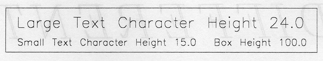
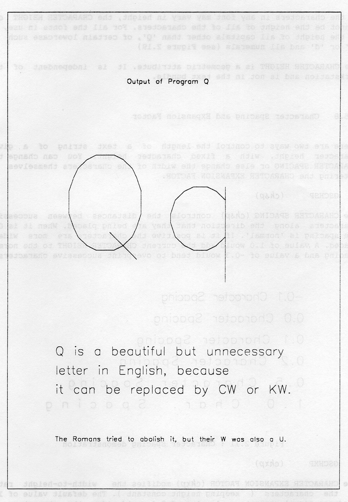
Example 2.8 shows how CHARACTER HEIGHT is used to control the size of characters in the text.
You may wish to control the size of the text. This is done through the CHARACTER HEIGHT attribute, which you can change with:
GSCHH (chh)
which changes the CHARACTER HEIGHT to chh. This is measured in GKS WORLD COORDINATES (the coordinates in use for graphics). For further details about coordinate systems see Chapter 3.
The default CHARACTER HEIGHT is 0.01 WORLD COORDINATE units. This is 1 of the default display height.
Figure 2.10 shows changing character heights.
      PROGRAM QDEM
*                                 GKS Example Program 2.8
*                                OPEN GKS, OPEN and ACTIVATE WORKSTATION. The
*                                parameters for OPEN GKS and OPEN WORKSTATION
*                                are system- and device- dependent; see Appendix B
*                                for details of the values which are valid on each
*                                system.
      CALL GOPKS (kerrfl, -1)
      CALL GOPWK (1 , kconid, kwtype)
      CALL GACWK (1)
*                                End of standard opening sequence
*----------------------------------------------------------------------------------
*                                Draw large 'Qq'
      CALL GSCHH  (0.2)
      CALL GTX (0.1, 0.5, 'Qq')
*                                Draw small text
      CALL GSCHH  (0.018)
      CALL GTX (0.1, 0.28,'Q is a beautiful but unnecessary')
      CALL GTX (0.1, 0.24,'letter in English, because')
      CALL GTX (0.1, 0.20,'it can be replaced by CW or KW.')
*                                Draw very small text (including heading)
      CALL GSCHH (0.01)
      CALL GTX (0.1, 0.10,
     :'The Romans tried to abolish it, but their W was also a U.')
      CALL GTX (0.25, 0.85,'Output of Program Q')
*----------------------------------------------------------------------------------
*                               Deactivate and close workstation, close GKS
      CALL GDAWK (1)
      CALL GCLWK (1)
      CALL GCLKS
      END
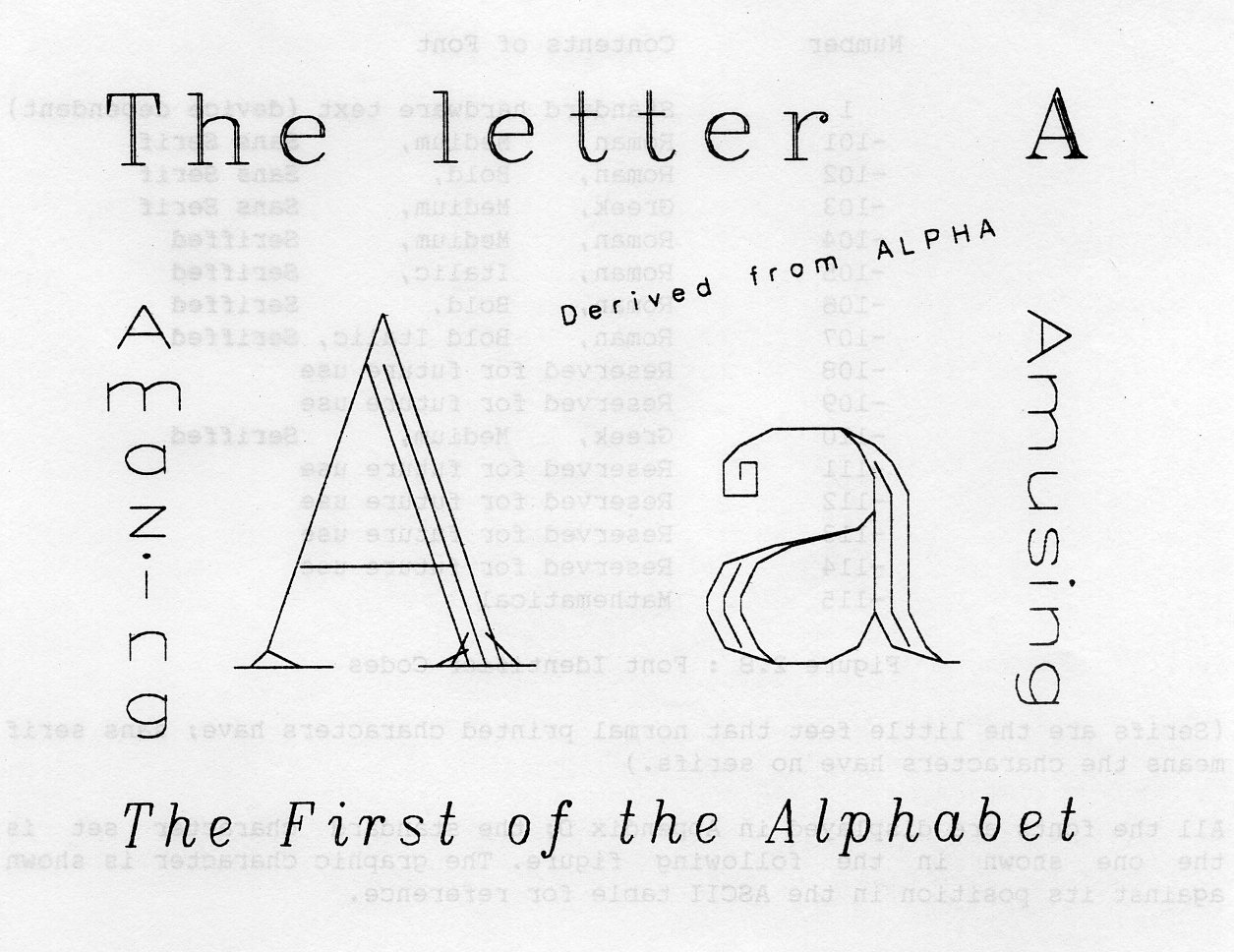
As the characters in any font may vary in height, the CHARACTER HEIGHT chh cannot be the height of all of the characters. For all the fonts in use, it is the height of all capitals other than 'Q', of certain lowercase such as 'b' or 'd' and all numerals (see Figure 2.19).
The CHARACTER HEIGHT is a geometric attribute. It is independent of the workstation and is not in the text bundle.
There are two ways to control the length of a text string of a given character height, with a fixed character height. You can change the CHARACTER SPACING or else change the width of the characters themselves by altering the CHARACTER EXPANSION FACTOR.
GSCHSP (chsp)
The CHARACTER SPACING (chsp) controls the distances between successive characters along the direction that they are being placed. When it is 0.0 the spacing is normal. If it is positive the characters are more widely spaced. A value of 1.0 would add the current CHARACTER HEIGHT to the normal spacing and a value of -0.3 would tend to overprint successive characters.
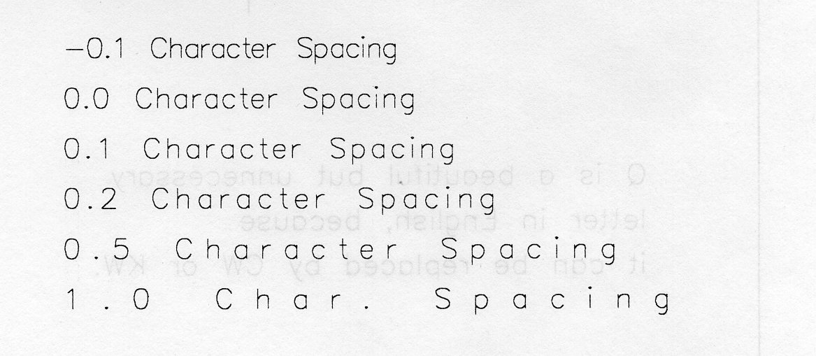
GSCHXP (chxp)
The CHARACTER EXPANSION FACTOR (chxp) modifies the width-to-height ratio of the characters ( keeping height constant). The default value of 1.0 produces normal characters. A value of 2.0 would widen the characters to twice their normal width and a value of 0.7 would narrow them down to 70% of their normal width.
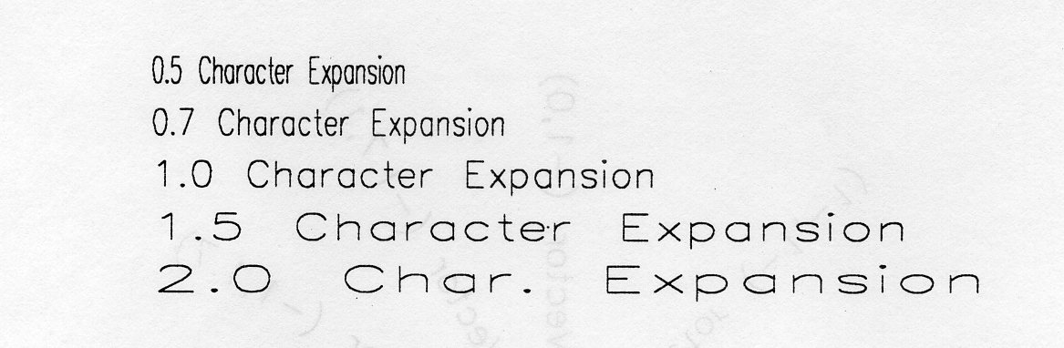
CHARACTER EXPANSION does not effect the spaces between the characters. For example suppose a string has a length of 100 when produced with normal character spacing and expansion. If the CHARACTER SPACING of the string is then raised to give it a length of 151, doubling the CHARACTER EXPANSION will not double the length, but change it to 251.
The CHARACTER EXPANSION and CHARACTER SPACING are not geometric attributes. A workstation may only support a limited number or range of character spacings or expansion factors, in which case the nearest available one is used. Both of these attributes are in the TEXT BUNDLE.
To use the character expansion and spacing to control the length of a string of text (eg, to fit it on a line), you use INQUIRE TEXT EXTENT (GQTXX, see section 8.4.1).
If you want your text to slope or point in any direction, then you can rotate the text by changing the CHARACTER UP-VECTOR:
GSCHUP (chux, chuy)
where (chux, chuy] is the new value for the CHARACTER UP-VECTOR.
This CHARACTER UP-VECTOR always points in the upward direction of the characters.
In the figure below strings are drawn at the CHARACTER UP-VECTOR shown. Each string starts at the same point with ... to prevent excessive overlap.
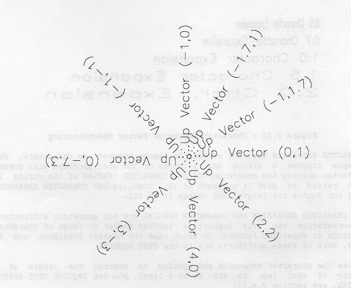
The CHARACTER UP-VECTOR is defined in terms of the current world coordinates. If X and Y have equal ranges (as in the default coordinate system), the values 2.0,2.0 would make the text slope 45 degrees downwards. Only the ratio of the two values is relevant: for example, 3.6,3.6 would have the same effect as 2.0,2.0.
This attribute is geometric and so is not in the text bundle.
You may want to rotate the text without also rotating the characters. This is possible if the rotation is a whole number of right angles and can be done by changing the TEXT PATH attribute. You can do it with routine:
GSTXP (jtxp)
The TEXT PATH (set to jtxp) must be one of the following:
GRIGHT   0 character 'n+1' right of character 'n' (default)
GLEFT    1 character 'n+1' left  of character 'n'
GUP      2 character 'n+1' above    character 'n'
GDOWN    3 character 'n+1' below    character 'n'
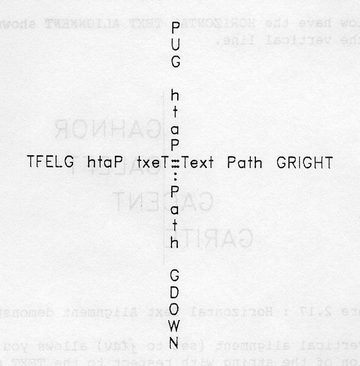
This attribute is geometric and is not in the text bundle.
Text is normally produced from the lower left of the string. However there are cases when you would want the text to be fixed at some other point in the string. You can do this by changing the TEXT ALIGNMENT.
GSTXAL (jtxalh, jtxalv)
With jtah you control the horizontal position of the string with respect to the TEXT point (px,py) given in the routine GTX. The horizontal alignment (set to jtah) can be one of the following:
GAHNOR 0   normal alignment (depends on TEXT PATH)
            = GALEFT if Text Path is GRIGHT
            = GARITE if Text Path is GLEFT
            = GACENT if Text path is GUP or GDOWN
GALEFT 1   align left end of string to TEXT point
GACENT 2   align centre of string to TEXT point
GARITE 3   align right end of string to TEXT point
The strings below have the HORIZONTAL TEXT ALIGNMENT shown and all have the TEXT point on the vertical line.
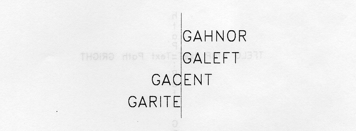
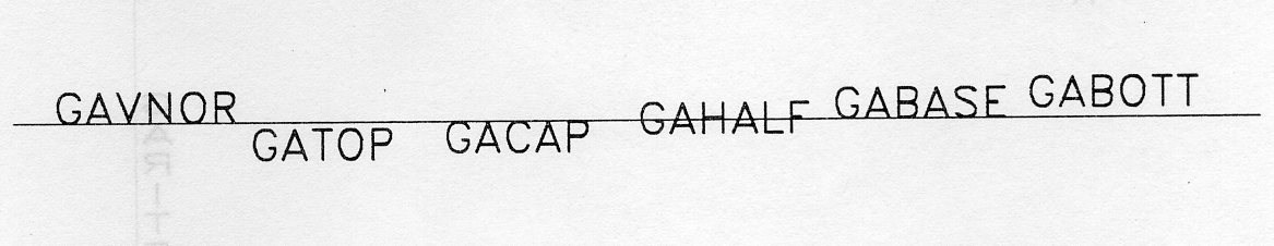
Similarly the vertical alignment (set to jtav) allows you to control vertical position of the string with respect to the TEXT point.
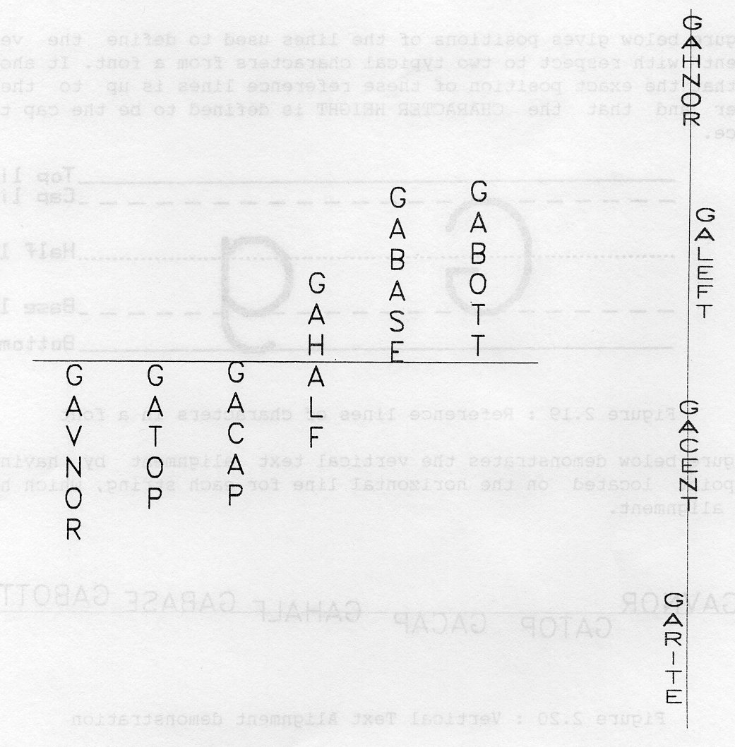
GAVNOR   0 normal alignment (=GABASE usually)
GATOP    1 align top of string to TEXT point
GACAP    2 align top of capital letters to TEXT point
GAHALF   3 align middle of characters to TEXT point
GABASE   4 align baseline of characters to TEXT point
GABOTT   5 align bottom of character box to TEXT point
The figure below gives positions of the lines used to define the vertical alignment with respect to two typical characters from a font. It should be noted that the exact position of these reference lines is up to the font designer and that the CHARACTER.HEIGHT is defined to be the cap to base distance.

The figure below demonstrates the vertical text alignment by having the text point located on the horizontal line for each string, which has the stated alignment.
For vertical text paths, the horizontal alignment remains horizontal. To control which end of a vertical text string is aligned with the text point/ you use the vertical alignment.
For Vertical text paths (GUP and GDOWN), the vertical alignment is defined so that the level of the text point is as follows:
GAVNOR 0 Start of string
GATOP  1 Top of TOP character
GACAP  2 Cap of TOP character
GAHALF 3 middle of character MID lines
GABASE 4 Base of BOTTOM character.
GABOTT 5 Bottom of BOTTOM character.
TEXT ALIGNMENT is geometric and so is not in the text bundle.
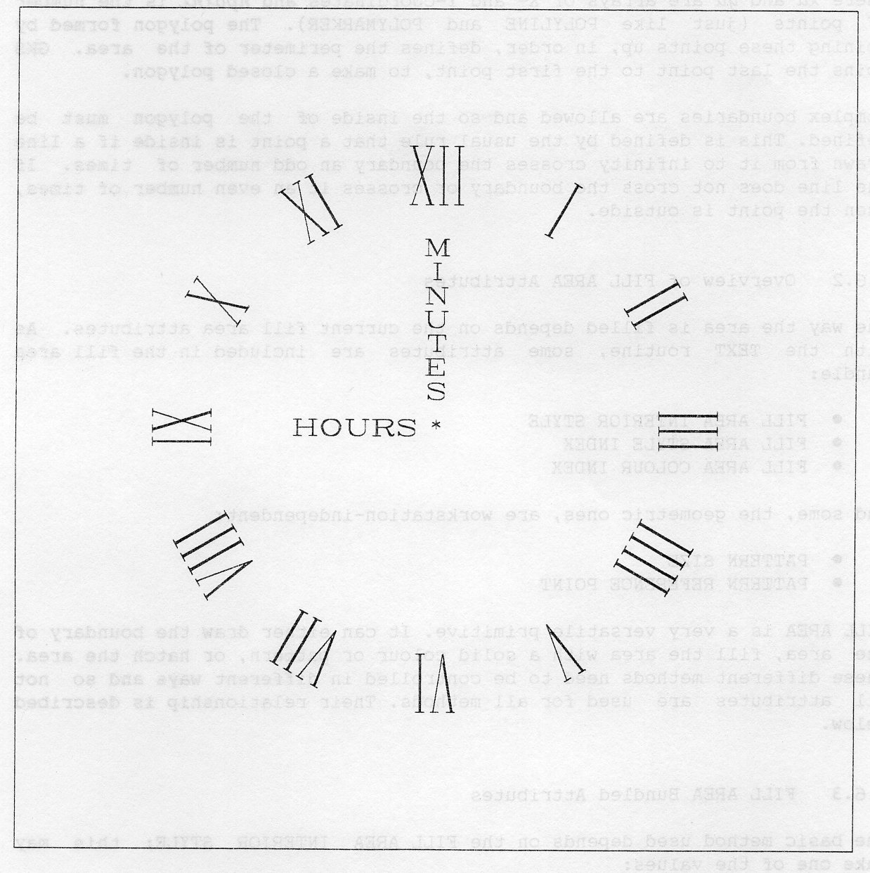
Example 2.9 shows how a number of the text attributes may be used individually.
      PROGRAM CLOCK
*                                 GKS Example Program 2.9
*                                 The following variable(s) are defined in the
*                                 included file
*                                 GINDIV, GSTRKP, GDOWN, GACENT, GATOP, GARITE, etc
*                                 include GKS parameter file - see Appendix B for details
      CHARACTER*39 NUM
      INTEGER NUMLEN(12), JASF(13), ICONID, IWTYPE, ISTART, IHOUR, IEND
      REAL HANGLE, HX, HY
      PARAMETER(HANGLE=3.14159/6.0)
      DATA NUM/'I II III IIII V VI VII VIII IX X XI XII'/
      DATA NUMLEN /1,2,3,4,1,2,3,4,2,1,2,3/
      DATA JASF /13*GINDIV/
*                                OPEN GKS, OPEN and ACTIVATE WORKSTATION. The
*                                parameters for OPEN GKS and OPEN WORKSTATION
*                                are system- and device- dependent; see Appendix B
*                                for details of the values which are valid on each
*                                system.
      CALL GOPKS (kerrfl, -1)
      CALL GOPWK (1 , kconid, kwtype)
      CALL GACWK (1)
*                                End of standard opening sequence
*----------------------------------------------------------------------------------
*                                Set ASPECT SOURCE FLAGS to INDIVIDUAL
      CALL GSASF (JASF)
*                                Set font
      CALL GSTXFP (-104,GSTRKP)
*                                Set attributes for numerals on clock face
      CALL GSCHH (0.07)
      CALL GSCHXP (0.5)
      CALL GSTXAL (GACENT,GATOP)
      ISTART = 1
*                                Loop to draw each Roman numeral appropriately sloped
      DO 10 IHOUR=1,12
*                                Calculate and set character up vector for numeral
      HX = SIN (IHOUR*HANGLE)
      HY = COS (IHOUR*HANGLE)
      CALL GSCHUP (HX,HY)
*                                Get numeral from numeral string and draw it
      IEND = ISTART + NUMLEN(IHOUR) - 1
      CALL GTX (0.35*HX + 0.5, 0.35*HY + 0.5,NUM(ISTART:IEND))
      ISTART = IEND + 2
  10  CONTINUE
*                                Set attributes and draw Hour hand
      CALL GSCHH(0.02)
      CALL GSCHXP (1.5)
      CALL GSCHSP (-0.1)
      CALL GSTXAL (GARITE,GAHALF)
      CALL GTX(0.5,0.5,'HOURS ')
*                               Set attributes and draw Minute hand
      CALL GSTXAL (GAHNOR,GABOTT)
      CALL GSTXP (GDOWN)
      CALL GTX(0.5,0.5,'MINUTES ')
*                               Set attributes and draw centre
      CALL GSTXAL (GACENT,GAHALF)
      CALL GSCHXP (1.0)
      CALL GTX(0.5,0.5,'*' )
*----------------------------------------------------------------------------------
*                               Deactivate and close workstation, close GKS
      CALL GDAWK (1)
      CALL GCLWK (1)
      CALL GCLKS
      END
In many applications, line drawings are insufficient and filled areas are required. In integrated circuit design, the content of each layer would be displayed by a collection of filled rectangles. More general shapes are required to be filled in animation applications. An area defined by a boundary may be filled with a colour or a pattern. You do this with FILL AREA:
GFA (npoint, xa, ya)
where xa and ya are arrays of X- and Y-coordinates and npoint is the number of points (just like POLYLINE and POLYMARKER). The polygon formed by joining these points up, in order, defines the perimeter of the area. GKS joins the last point to the first point, to make a closed polygon.
Complex boundaries are allowed and so the inside of the polygon must be defined. This is defined by the usual rule that a point is inside if a line drawn from it to infinity crosses the boundary an odd number of times. If the line does not cross the boundary or crosses it an even number of times, then the point is outside.
The way the area is filled depends on the current fill area attributes. As with the TEXT routine, some attributes are included in the fill area bundle:
and some, the geometric ones, are workstation-independent:
FILL AREA is a very versatile primitive. It can either draw the boundary of the area, fill the area with a solid colour or pattern, or hatch the area. These different methods need to be controlled in different ways and so not all attributes are used for all methods. Their relationship is described below.
The basic method used depends on the FILL AREA INTERIOR STYLE; this may take one of the values:
GHOLLO   (0) the boundary is drawn, but the area not filled;
GSOLID   (l) the whole area is filled;
GPATTR   (2) the area is filled by repeating a pattern in both X and Y;
GHATCH   (3) the area is filled with a hatch style.
If the style requires a single colour (ie GHOLLO, GSOLID, GHATCH) then that is selected by the FILL AREA COLOUR INDEX. If the style can be subdivided (for example, which pattern for GPATTR or which hatch for GHATCH) then this is selected by the FILL AREA STYLE INDEX. In other cases these two attributes are ignored.
All these attributes are included in the FILL AREA BUNDLE. The two routines for handling FILL AREA BUNDLES are SET FILL AREA INDEX and SET FILL AREA REPRESENTATION:
GSFAI (kfai)
This specifies that subsequent fill areas are to be produced according to the representation of bundle kfai. If you wish to change the representation, you call
GSFAR   (kwkid, kfai, jstyle, kstylei, kfacol)
(kujkM, k$cU, j
which changes the representation of fill area bundle kfai, on workstation kwkid; jstyle is the interior style, kstyli is the style index and kfacol the colour index. For some workstations, this will cause all output created with this index to be modified (see Section 2.11, Implicit Regeneration).
All workstations must support interior style GHOLLO but the other interior styles are optional, although if provided they must be provided as described. If GPATTR is supported, then the patterns may be either predefined or defined by you. This is described in more detail in the next section. If GHATCH is supported then all the hatch styles are defined by the implementation and may not be changed by you.
Example 2.10 illustrates a number of interior styles.
      PROGRAM FASTY
*                                 GKS Example Program 2.10
*                                 The following variable(s) are defined in the
*                                 included file
*                                 GSOLID, GPATTR, GHOLLO
*                                 include GKS parameter file - see Appendix B for details
*                                 Data for Ship's Outline
      INTEGER NSHIP
      PARAMETER (NSHIP = 18)
      REAL XSHIP(NSHIP), YSHIP(NSHIP)
      DATA XSHIP/0.20,0.10,0.40,0.42,0.50,0.52,0.58,0.56,0.64,
     :          0.66,0.72,0.70,0.78,0.78,0.92,0.92,0.90,0.20/
     :     YSHIP/0.12,0.22,0.20,0.26,0.26,0.32,0.32,0.26,0.26,
     :           0.32,0.32,0.26,0.26,0.20,0.20,0.14,0.12,0.12/
*                                OPEN GKS, OPEN and ACTIVATE WORKSTATION. The
*                                parameters for OPEN GKS and OPEN WORKSTATION
*                                are system- and device- dependent; see Appendix B
*                                for details of the values which are valid on each
*                                system.
      CALL GOPKS (kerrfl, -1)
      CALL GOPWK (1 , kconid, kwtype)
      CALL GACWK (1)
*                                End of standard opening sequence
*----------------------------------------------------------------------------------
*                                Set Fill Area Representations for different interior
*                                styles
      CALL GSFAR (1, 1, GSOLID,  0, 1)
      CALL GSFAR (1, 2, GHATCH, -1, l)
      CALL GSFAR (1, 3, GHOLLO,  0, 1)
*                                Draw three ships at different sizes in different
*                                styles
      CALL GSFAI (l)
      CALL GFA (NSHIP, XSHIP, YSHIP)
      DO 10 1=1,NSHIP
      XNSHIP(I) = XSHIP(I) * 0.5 + 0.5
      YNSHIP(I) - YSHIP(I) * 0.5 + 0.5
   10 CONTINUE
      CALL GSFAI (2)
      CALL GFA (NSHIP, XNSHIP, YNSHIP)
      DO 20 1=1,NSHIP
       XNSHIP(I) = XSHIP(I) * 0.375
       YNSHIP(I) = YSHIP(I) * 0.375 + 0.75
   20 CONTINUE
      CALL GSFAI (3)
      CALL GFA (NSHIP, XNSHIP, YNSHIP)
*----------------------------------------------------------------------------------
*                               Deactivate and close workstation, close GKS
      CALL GDAWK (1)
      CALL GCLWK (1)
      CALL GCLKS
      END
If the style GPATTR is selected then the area is filled with a pattern. This may be either predefined or defined by you. On workstations supporting patterns at least one will be predefined. A pattern is specified by a two dimensional array of colour indices, which is why for this style the FILL AREA COLOUR INDEX is ignored. The precise way in which this array is mapped into the area to be filled is determined by the two workstation independent attributes of fill area: PATTERN SIZE and PATTERN REFERENCE POINT. (Note that many drivers do not support pattern size; see Appendix C for details). The area is filled as if the pattern array was located with its lower left corner at the pattern reference point. It is then repeated in both the X and Y directions. The fill area is then filled with the colour indices of the pattern which cover the area. This means that two adjacent fill areas which are filled with the same values for pattern reference point will appear as if they had been one fill area, ie the pattern will continue across the common boundary. These attributes may be set by the routines:
GSPA     (szx, szy)
GSPARF   (nfx, nfy)
where szx and szy are the size of the pattern expressed in the current coordinate system, and nfx and nfy give the reference point for the pattern also in the current coordinate system.
The patterns, themselves, may be set by:
GSPAR (kwkid, kpai, mx, my, isc, isn, nx, ny, kcola)
which sets the pattern for style index kpai, on workstation kwkid; mx and my are the dimensions of the colour index array kcola specifying the pattern. The pattern may be contained in a submatrix of the colour index array: isc and isr specify the indices of the start column and start row, and nx and ny specify the numbers of rows and columns. For some workstations, this will cause all output created with this index to be modified (see Section 2.11, Implicit Regeneration).
In order that the array does not have to precisely match the size of the data, mx specifies the size of the first dimension of kcola. (of course, this must be greater than or equal to nx).
In order to allow for adjacent filled areas, pattern filling includes the left hand and top boundaries, but not the right hand and bottom boundaries. This means that if you draw a rectangle with thin lines, and then fill it with a pattern, the left and top lines are overwritten by the pattern. If you want a drawn boundary round the area, you should draw it after filling the area.
Each of the attributes available in the fill area bundle may be set individually, as long as SET ASPECT SOURCE FLAGS has been called to ensure that the individual attributes will be used. The routines are SET FILL AREA INTERIOR STYLE, SET FILL AREA STYLE INDEX and SET FILL AREA COLOUR INDEX:
GSFAIS   (jstyle)
GSFASI   (kstyli)
GSFACI   (kfacol)
The default individual fill area interior style has value GHOLLO.
In addition to all the drawing routines outlined so far, GKS provides an imaging capability. Whether the image data comes from an astronomical telescope or a CRT scanner, GKS provides a facility to display this data.
This is the routine CELL ARRAY:
GCA (px, py, qx, qy, lx, ly, isc, isr, mx, my, kcola)
where kcola is a lx by ly array of colour indices representing the image data. These point to the colour table on each workstation. Thus the data may appear as a greyscale image on a monochrome display or as a false colour image on a colour display. The image is stored in kcola such that the first dimension increases as X increases and the second dimension increases as Y decreases. Two points P,Q are specified by (px, py) and (qx, qy) determine the size of the displayed cell array. They define a rectangle parallel to the axes of the current coordinate system where P is the upper left corner and Q is the lower right corner. The array of cells (whose colours are determined by the colour index array) is scaled to precisely fill this rectangle. This means that the cells may not correspond precisely to device pixels. (If an integer mapping to device pixels is required, care should be taken in setting up the coordinate systems - see Chapter 3.)
The advantage of this is that the cell array has a well defined coordinate system so that if, for example, it is desired to plot contours on top of the cell array it may be easily accomplished.
It may be that only a submatrix of the array kcola is required to define the image; isc and isr specify the indices of the start column and start row, and mx and my specify the number of rows and columns to be used.
On some workstations it is difficult to produce a cell array image, in which case a rectangle representing the outline of the array is shown instead.
Since the colour index array is specified by the cell array routine, as are the points P and Q, CELL ARRAY has no attributes at all.
In Example 2.11 a chessboard pattern is output. The CELLEX data file has the form of a matrix of ones and zeros:
01010101
10101010
01010101
10101010
01010101
10101010
01010101
10101010
Colour index 0 is shown as white, and colour index 1 as black in the example output.
      PROGRAM CELLEX
*                                 GKS Example Program 2.11
      INTEGER KCOLA(8,8)
*                                 FORTRAN unit number for input
      INTEGER IUNIT
*                                 The FORTRAN unit number for input is system-
*                                 dependent; see Appendix B for details
*                                  of the values which are valid on each system.
      PARAMETER (IUNIT = fstiun)
*                                OPEN GKS, OPEN and ACTIVATE WORKSTATION. The
*                                parameters for OPEN GKS and OPEN WORKSTATION
*                                are system- and device- dependent; see Appendix B
*                                for details of the values which are valid on each
*                                system.
      CALL GOPKS (kerrfl, -1)
      CALL GOPWK (1 , kconid, kwtype)
      CALL GACWK (1)
*                                End of standard opening sequence
*----------------------------------------------------------------------------------
*                                Read data row by row
      OPEN (UNIT=IUNIT, FILE='datafn' , STATUS='OLD' )
      READ (IUNIT, '(8I1)') KCOLA
*                                Draw cell array
      CALL GCA (0.4, 0.6, 0.6, 0.4, 8, 8, 1, 1, 8, 8, KCOLA)
*----------------------------------------------------------------------------------
*                               Deactivate and close workstation, close GKS
      CALL GDAWK (1)
      CALL GCLWK (1)
      CALL GCLKS
      END
You have seen all the output primitives which will always be available. However, some workstations may have output capabilities which cannot be addressed by these primitives, for example circle or ellipse drawing. GKS provides access to these capabilities in a uniform manner but does not guarantee what output will be produced nor that it will be produced on every workstation. If a workstation does not have the appropriate capability an error will be produced. Hence, use of these capabilities limits the portability of an application program.
These capabilities are accessed via the GENERALIZED DRAWING PRIMITIVE or GDP:
GGDP (npoint, xa, ya, kgdpid, lgdpdn, gdpdn)
As with POLYLINE, POLYMARKER and FILL AREA, npoint positions are given in the xa and ya arrays. The particular GDP is selected by kgdpid.
The basic GDP identifiers are:
-1 Arc, unstyled
-2 Arc (chord) with interior styled
-3 Arc (pie) with interior styled
-4 Arc (circle) with interior styled
Full details of those that are available are listed in Appendix G, and Appendix C gives details of which GDPs are supported on each workstation. Further information may be necessary and this is passed via a data record gdpgn which is an array of CHARACTER*80 elements of dimension lgdpdn. Note that these are RAL GKS dependent; if you use them you will reduce the portability of your program.
Since a GDP may take quite different forms depending on which particular GDP is used (as selected by kgdpid), it is difficult to define a set of attributes for a GDP. One GDP may be essentially a polyline (for example, an arc) whereas another may be essentially a fill area (for example, a sector of a pie chart). As a consequence, a GDP uses one or more of the sets of attributes defined for the other primitives. The sets of attributes used by a GDP are defined for each particular GDP. For example, an arc would use the polyline attributes whereas the pie chart sector would use the fill area attributes. The attributes are used in precisely the same way as for the primitives to which they belong and, where appropriate, may be used in BUNDLED or INDIVIDUAL mode depending on the setting of the corresponding ASPECT SOURCE FLAGS.
In example 2.12 a GDP to draw a filled sector is used to generate a pie chart.
      PROGRAM GDPEX
*                                 GKS Example Program 2.12
*                                 The following variable(s) are defined in the
*                                 included file
*                                 GHATCH
*                                 include GKS parameter file - see Appendix B for details
      CHARACTER*80 NODAT(l)
      REAL XC, YC, RADIUS
      REAL XA(3), YA(3), THETAD(3)
      DATA XC, YC, RADIUS/0.5, 0.5, 0.375/
      DATA THETAD/150.0, 115.0, 95.0/
*                                OPEN GKS, OPEN and ACTIVATE WORKSTATION. The
*                                parameters for OPEN GKS and OPEN WORKSTATION
*                                are system- and device- dependent; see Appendix B
*                                for details of the values which are valid on each
*                                system.
      CALL GOPKS (kerrfl, -1)
      CALL GOPWK (1 , kconid, kwtype)
      CALL GACWK (1)
*                                End of standard opening sequence
*----------------------------------------------------------------------------------
*                                Calculate PI
      PI = 4.0 * ATAN (1.0)
*                                Set Representations for 3 sectors of pie chart
      CALL GSFAR (1, 1, GHATCH, -1, 1)
      CALL GSFAR (1, 2, GHATCH, -2, 1)
      CALL GSFAR (1, 3, GHATCH, -3, 1)
*                                Calculate first point of first sector TH = 0.0
      XA(1) = XC + RADIUS * SIN (TH)
      YA(1) = YC + RADIUS * COS (TH)
*                                Draw three sectors of pie chart
      DO 20 I=1,3
*                                Calculate half sector angle in radians
      THETAR = THETAD(I) * PI / 360.0
*                                Calculate two other points for sector
      DO 10 J=2,3
       TH = TH + THETAR
       XA(J) = XC + RADIUS * SIN (TH)
       YA(J) = YC + RADIUS * COS (TH)
  10  CONTINUE
*                                Set fill area bundle index
      CALL GSFAI (I)
*                                Draw sector (no data in data record)
      CALL GGDP (3, XA, YA, -3, 1, NODAT)
*                               Set first point of next sector to last point of this
      XA(1) = XA(3)
      YA(1) = YA(3)
   20 CONTINUE
*----------------------------------------------------------------------------------
*                               Deactivate and close workstation, close GKS
      CALL GDAWK (1)
      CALL GCLWK (1)
      CALL GCLKS
      END
In section 2.2, you saw that GKS provides two ways of specifying attributes, BUNDLED and INDIVIDUAL. Although they are each used for a variety of purposes, the simplest explanation is that BUNDLED attributes ensure that you get distinguishable output from different bundles, whereas INDIVIDUAL attributes attempt the closest match possible to the attributes you specified.
GKS has no way of telling whether you want to use BUNDLED or INDIVIDUAL attributes; you have to specify this with SET ASPECT SOURCE FLAGS:
GSASF (jasf)
jasf is an array of 13 flags, each of which is set to either GINDIV (value 1, for INDIVIDUAL) or GBUNDL (value 0, for BUNDLED). There is one flag for each attribute, according to the following list:
Element     Attribute
1            Linetype
2            Linewidth Scale Factor
3            Polyline Colour Index
4            Markertype
5            Marker Size Scale Factor
6            Polymarker Colour Index
7            Text Font and Precision
8            Character Expansion Factor
9            Character Spacing
10           Text Colour Index
11           Fill Area Interior Style
12           Fill Area Style Index
13           Fill Area Colour Index
An example of setting ASF's can be seen in Example 2.15.
There are several situations where colour has to be specified in GKS. These include the colour for POLYLINE, POLYMARKER and text primitives, sets of colours for FILL AREA patterns and the individual elements of CELL ARRAY. In order that device independence is possible, in GKS you specify all colours by indices that point into a colour table; there is a separate colour table for each workstation. On a 16 colour terminal, the colour table might be:
Colour Index  Red  Green  Blue  Usual Name
     0        0.0   0.0   0.0    black
     1        1.0   1.0   1.0    white
     2        1.0   0.0   0.0    red
     3        0.0   1.0   0.0    green
     4        0.0   0.0   1.0    blue
     5        1.0   1.0   0.0    yellow
     6        0.0   0.0   1.0    cyan
     7        1.0   0.0   1.0    magenta
     8        0.0   0.0   0.0    black
     9        0.2   0.2   0.2    grey 3/15
    10        0.33  0.33  0.33   grey 5/15
    11        0.47  0.47  0.47   grey 7/15
    12        0.6   0.6   0.6    grey 9/15
    13        0.73  0.73  0.73   grey 11/15
    14        0.87  0.87  0.87   grey 13/15
The colour tables contain, for each index, the intensity levels for red, green and blue components of the colour. To select a different colour, you may therefore just select a different colour index. One inquiry function allows you to check whether the device you are driving supports colour (INQUIRE COLOUR FACILITIES, GQCF). Other inquiry functions allow you to investigate the range of colours available.
A simple use of different colours for some lines of text is shown in example 2.13. This example assumes that you are using a device which is known to have colour and that text bundles 1, 2 and 3 produce text in three different colours. The change of colour is achieved very simply by SET TEXT INDEX.
Example 2.14 shows a more positive approach, where you SET COLOUR REPRESENTATION (GSCR) and then use the colours you have set. You still need to check that your device supports enough colours and then SET TEXT REPRESENTATIONS so that selecting different text bundles selects different colours.
      PROGRAM CONCOL
*                                OPEN GKS, OPEN and ACTIVATE WORKSTATION. The
*                                parameters for OPEN GKS and OPEN WORKSTATION
*                                are system- and device- dependent; see Appendix B
*                                for details of the values which are valid on each
*                                system.
      CALL GOPKS (kerrfl, -1)
      CALL GOPWK (1 , kconid, kwtype)
      CALL GACWK (1)
*                                End of standard opening sequence
*----------------------------------------------------------------------------------
*                                Set character height
      CALL GSCHH (0.1)
*                                Output three lines of text, each in a
*                                different colour by changing bundle index
      CALL GSTXI (1)
      CALL GTX   (0.1, 0.7, 'Pretty')
      CALL GSTXI (2)
      CALL GTX   (0.1, 0.5, 'Coloured')
      CALL GSTXI (3)
      CALL GTX   (0.1, 0.3, 'Text')
*----------------------------------------------------------------------------------
*                               Deactivate and close workstation, close GKS
      CALL GDAWK (1)
      CALL GCLWK (1)
      CALL GCLKS
      END
      PROGRAM COLREP
*                                 GKS Example Program 2.14
*                                 The following variable(s) are defined in the
*                                 included file
*                                 GCOLOR, GSET
*                                 include GKS parameter file - see Appendix B for details
*                                OPEN GKS, OPEN and ACTIVATE WORKSTATION. The
*                                parameters for OPEN GKS and OPEN WORKSTATION
*                                are system- and device- dependent; see Appendix B
*                                for details of the values which are valid on each
*                                system.
      CALL GOPKS (kerrfl, -1)
      CALL GOPWK (1 , kconid, kwtype)
      CALL GACWK (1)
*                                End of standard opening sequence
*----------------------------------------------------------------------------------
*                                Check that the workstation supports colour
      CALL GQCF (kwtype, KERROR, NCOL, JCOLAV, NPCI)
      IF (JCOLAV .EQ. GCOLOR) THEN
*                                Device supports colour: check number of colours
      IF (NCOL .GE. 3) THEN
*                                Set representation for colour indices 1,2, 3
        CALL GSCR (1, 1, 1.0, 0.0, 0.0)
        CALL GSCR (1, 2, 0.0, 1.0, 0.0)
        CALL GSCR (1, 3, 0.0, 0.0, 1.0)
*                                Inquire text representations and reset colour
*                                for text indices 1,2,3 to 1,2,3
        DO 10 KTXI=1,3
          CALL GQTXR (1, KTXI, JTYPE, KERROR, KFONT, JPREC, CHXP, CHSP, KTXCOL)
          IF (KTXCOL .NE. KTXI) CALL GSTXR (1, KTXI, KFONT, JPREC, CHXP, CHSP, KTXCOL)
   10   CONTINUE
*                                Now produce text output as before
        CALL GSCHH (0.1)
        CALL GSTXI (1)
        CALL GTX (0.1, 0.7, 'Pretty')
        CALL GSTXI (2)
        CALL GTX (0.1, 0.5, 'Coloured')
        CALL GSTXI (3)
        CALL GTX (0.1, 0.3, 'Text')
      ENDIF
      ELSE
*                                Device doesn't support colour
      WRITE (kerrfl,*) 'Example COLREP: workstation does not',
     :' support colour*
      ENDIF
*----------------------------------------------------------------------------------
*                               Deactivate and close workstation, close GKS
      CALL GDAWK (1)
      CALL GCLWK (1)
      CALL GCLKS
      END
On some devices (such as most pen plotters) the range of colours may be fixed and the above mechanism is fine. On others, including many raster displays, the device is capable of displaying a large number of different colours (perhaps 4096) but can only display a much smaller number (perhaps 16) simultaneously. In this case the colour table will have as many entries as the device has simultaneous colours. You can still access the full range of colours from GKS by redefining the colour representations, in other words the colour table entries.
The final colour example (2.15) is the most direct method, whereby you set the colour index directly. For this, the ASPECT SOURCE FLAG for TEXT COLOUR INDEX has to have been set to INDIVIDUAL.
      PROGRAM DIRCOL
*                                 GKS Example Program 2.15
*                                 The following variable(s) are defined in the
*                                 included file
*                                 GINDIV
*                                 include GKS parameter file - see Appendix B for details
*                                 Set up parameters with names for the ASFs
      INTEGER    GALN,      GALWSC,    GAPLCI,   GAMK,     GAMKSC
      PARAMETER (GALN=1,    GALWSO2,  GAPLCI=3, GAMK=4,   GAKKSO5)
      INTEGER    GAPMCI,    GATXFP,    GACHXP,   GACHSP,   GATXCI
      PARAMETER (GAPMCI=6,  GATXFP=7,  GACHXP=8, GACHSP=9, GATXCI=10)
      INTEGER    GAFAIS,    GAFASI,    GAFACI
      PARAMETER (GAFAIS=11, GAFASI=12, GAFACI=13)
*                                JASF is an array that holds the ASFS INTEGER JASF(13)
*                                OPEN GKS, OPEN and ACTIVATE WORKSTATION. The
*                                parameters for OPEN GKS and OPEN WORKSTATION
*                                are system- and device- dependent; see Appendix B
*                                for details of the values which are valid on each
*                                system.
      CALL GOPKS (kerrfl, -1)
      CALL GOPWK (1 , kconid, kwtype)
      CALL GACWK (1)
*                                End of standard opening sequence
*----------------------------------------------------------------------------------
*                                Check that the workstation supports colour
      CALL GQCF (kwtype, KERROR, NCOL, JCOLAV, NPCI)
      IF (JCOLAV .EQ. GCOLOR) THEN
*                                Device supports colour: check number of colours
      IF (NCOL .GE. 3) THEN
*                                Set ASPECT SOURCE FLAG for TEXT COLOUR
*                                INDEX to INDIVIDUAL
      CALL GQASF (KERROR, JASF)
      JASF(GATXCI) = GINDIV
      CALL GSASF (JASF)
*                                Now set colour representations
      CALL GSCR (1, 1, 1.0, 0.0, 0.0)
      CALL GSCR (1, 2, 0.0, 1.0, 0.0)
      CALL GSCR (1, 3, 0.0, 0.0, 1.0)
*                                Now proceed as before, setting text
*                                colour index before each line of text
      CALL GSCHH (0.1)
      CALL GSTXCI (l)
      CALL GTX (0.1, 0.7, 'Pretty')
      CALL GSTXCI (2)
      CALL GTX (0.1, 0.5, 'Coloured')
      CALL GSTXCI (3)
      CALL GTX (0.1, 0.3, 'Text')
      ENDIF
      ELSE
*                                Device doesn't support colour
      WRITE (kerrfl,*) 'Example DIRCOL: workstation does not',
     :' support colour*
      ENDIF
*----------------------------------------------------------------------------------
*                               Deactivate and close workstation, close GKS
      CALL GDAWK (1)
      CALL GCLWK (1)
      CALL GCLKS
      END
Changing the representation on a workstation for a primitive, pattern, or colour index that has already been used in the picture should cause all primitives that have been drawn with that index as attribute to take on the new representation.
On some displays, for instance storage tubes or pen plotters, the whole picture would have to be redrawn. A refresh display, on the other hand, could probably perform this change immediately. You can find out whether implicit regeneration is required for a workstation if you use inquiry functions (Sections 8.3, 8.4).
For more information on deferral and implicit regeneration, see Sections 6.9 and 6.10.
Chapter 2 has described the six output functions in GKS. In all cases some coordinate information is specified, either a single point {for TEXT) or an array of points (for all the others). All these points are said to be in WORLD COORDINATES (WC).
You can set the limits of the world coordinates you want to use by calling SET WINDOW:
GSWN (ktnn, xmin, xmax, ymin, ymax)
where ktnn indicates which world coordinate system is being used; there will be a more detailed description later - for the moment it is sufficient to know that 1 is always a legal value here. The xmin, xmax, ymin, ymax values specify the left, right, bottom and top limits of the world coordinate system.
Suppose you want to draw a diagonal line from (-5.0,100.0) to (0.0,105.0). You could specify a world coordinate system in which the line went from one corner to the other as follows:
CALL GSWN (1, -5.0,0.0, 100.0,105.0)
Here the first parameter specifies the world coordinate system. Before drawing anything you must select this coordinate system by calling SELECT NORMALIZATION TRANSFORMATION:
GSELNT (ktnn)
The value ktnn selects a particular world coordinate system to be the current one for output.
To draw your line, the code would just be:
      REAL X(2),Y(2)
      DATA X/-5.0,0.0/
      DATA Y/100.0,105.0/
      CALL GSWN(1, -5.0,0.0, 100.0,105.0)
      CALL GSELNT(l)
      CALL GPL(2,X,Y)

Obviously only the diagonal line has actually been drawn by the example. It will be apparent by now that world coordinates are Cartesian. If the application stores the data in some other form, for example polar or spherical coordinates, then the program must convert these to world coordinates before drawing anything using GKS.
In addition GKS requires that X increases to the right and Y increases towards the top, as we made sure in the example. This is shown in the figure:
So the call:
CALL GSWN(1, -5.0, 0.0, 105.0, 100.0)
is wrong because the Y limits are the wrong way round.
The X and Y limits together define a WINDOW (hence the GKS name SET WINDOW). Like a real-life window, you can imagine looking through the GKS window at a view of your data.
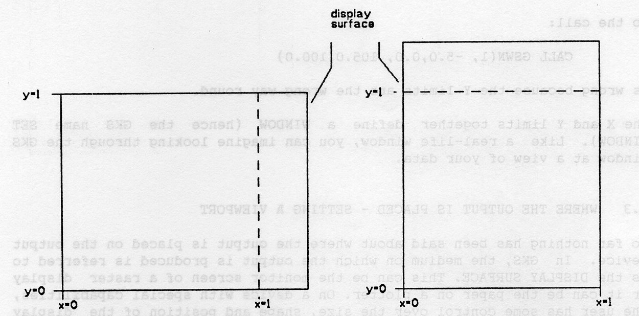
So far nothing has been said about where the output is placed on the output device. In GKS, the medium on which the output is produced is referred to as the DISPLAY SURFACE. This can be the monitor screen of a raster display or it can be the paper on a plotter. On a device with special capabilities, the user has some control over the size, shape and position of the display surface.
By default the output is fitted within the largest square on the display surface. The window limits are mapped to the limits of this square. Thus the diagonal line in the last example would actually go from corner to corner of a square on the display surface. However we would like to have more control over where the output goes.
It might seem that this has to be done using the coordinates of the device and of course devices come in many shapes, sizes and resolutions. If this were true, the routine calls would have to be altered whenever the program was run on another device. It is one of the aims of GKS that this should not be necessary.
Instead GKS provides a NORMALIZED device coordinate system (NDC). By default a unit square (0.0 to 1.0 in each of X and Y) is mapped to the display surface. If the device has an oblong display surface, this square is located in the bottom left as in the following figure.
To position the output, SET VIEWPORT can be used:
GSVP (ktnn, xmin, xmax, ymin, ymax)
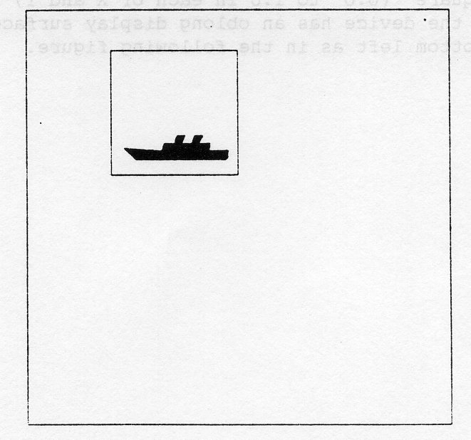
This specifies within the total unit square a rectangle (referred to as a viewport), whose limits in X are xmin and xmax and in Y are ymin and ymax. For example, to specify that output is to use a small square on the top left the following could be used:
CALL GSVP(1, 0.2,0.5, 0.6,0.9)
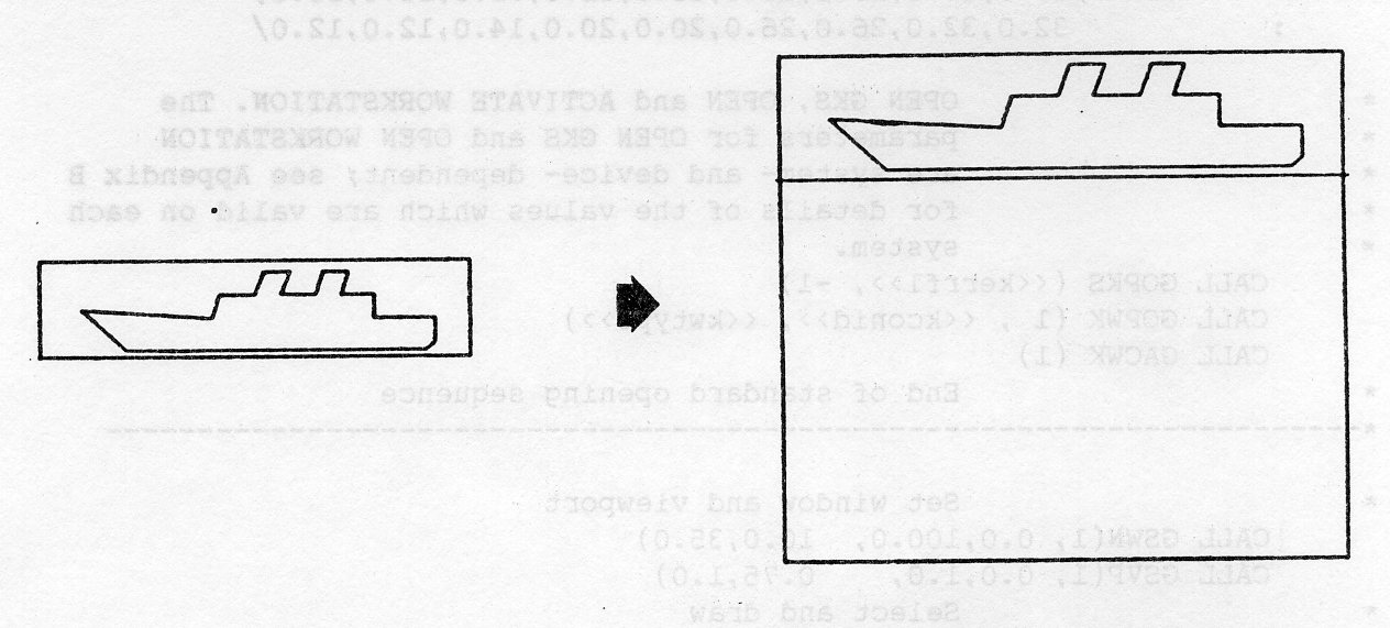
You can now place the ship in different places on the display surface. First note that the range of values in the ship is as follows:
Range in X 10.0 to 92.0
Range in Y 12.0 to 32.0
In the following example, you specify a window that includes the whole of the ship and map it to a viewport in the top half of the screen.
      PROGRAM WV
*                                 GKS Example Program 3.1
*                                 Data for Ship's Outline
      INTEGER NSHIP
      PARAMETER (NSHIP = 18)
      REAL XSHIP(NSHIP), YSHIP(NSHIP)
      DATA XSHIP/0.20,0.10,0.40,0.42,0.50,0.52,0.58,0.56,0.64,
     :          0.66,0.72,0.70,0.78,0.78,0.92,0.92,0.90,0.20/
     :     YSHIP/0.12,0.22,0.20,0.26,0.26,0.32,0.32,0.26,0.26,
     :           0.32,0.32,0.26,0.26,0.20,0.20,0.14,0.12,0.12/
*                                OPEN GKS, OPEN and ACTIVATE WORKSTATION. The
*                                parameters for OPEN GKS and OPEN WORKSTATION
*                                are system- and device- dependent; see Appendix B
*                                for details of the values which are valid on each
*                                system.
      CALL GOPKS (kerrfl, -1)
      CALL GOPWK (1 , kconid, kwtype)
      CALL GACWK (1)
*                                End of standard opening sequence
*----------------------------------------------------------------------------------
*                                Set window and viewport
      CALL GSWN(1, 0.0,100.0,  10.0,35.0)
      CALL GSVP(1, 0.0,1.0,    0.75,1.0)
*                                Select and draw
      CALL GSELNT(l)
      CALL GPL(NSHIP,XSHIP,YSHIP)
*----------------------------------------------------------------------------------
*                               Deactivate and close workstation, close GKS
      CALL GDAWK (1)
      CALL GCLWK (1)
      CALL GCLKS
      END
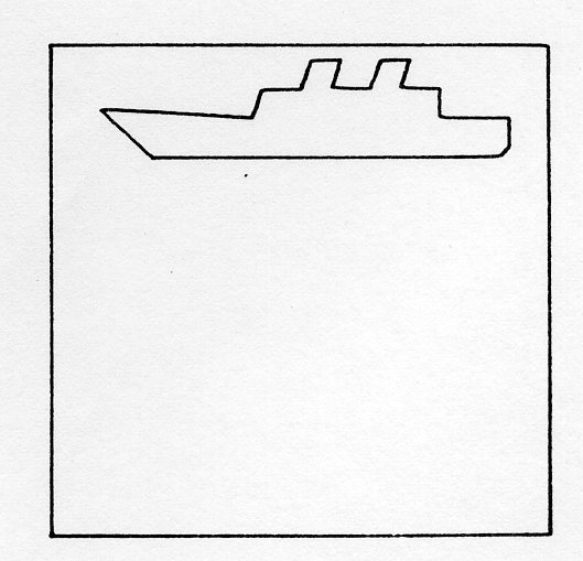
If you had wanted to place the ship at the bottom of the display surface (Y ranging from 0 to 0.25), you could simply have given different values to the SET VIEWPORT call:
CALL GSVP(1, 0.0,1.0, 0.0,0.25)
Since points are transformed to NORMALIZED device coordinates the transformation described is referred to as a NORMALIZATION TRANSFORMATION.
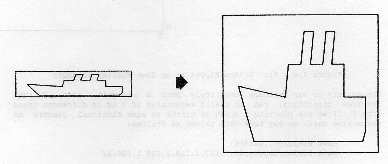
In the last example, the window and viewport were carefully chosen so that their X:Y ratios were the same - 4:1 in both cases. This was to preserve the shape of the ship when it was plotted. If the window with its 4:1 ratio had been mapped onto the default NDC square, the ship would have become squat:
Likewise if the viewport were a long narrow band, the ship would have become more like an ocean liner:
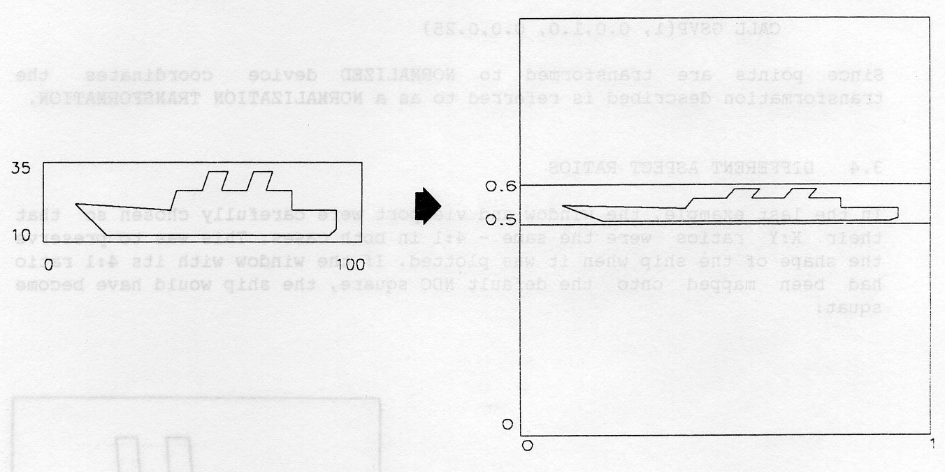
The ability to map a window completely onto a viewport, even if that involves distortion, can be useful especially if X is in different units from Y. If we are plotting a graph of births in some fictional country on successive days, we may have data values as follows:
      REAL BIRTHS(6),DAYS(6)
      DATA BIRTHS/102.0,140.7,120.3,119.2,119.1,120.1/
      DO 100 J=l,6
100   DAYS(J)=FLOAT(J)
The window can go from 0 to 7 in X and from 0 to 150 in Y:
CALL GSWN(1, 0.0,7.0, 0.0,150.0)
and the viewport can be the default 0 to 1 in each of X and Y. We can now plot the data points as follows:
CALL GPM(6,DAYS,BIRTHS)
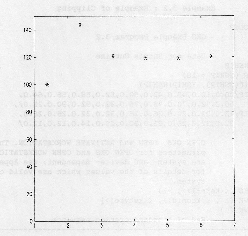
Note that the scale in world coordinates and axes have been added to the diagram.
Until now the examples have carefully set the window so that all the points lie within it. To see an enlarged view of part of the ship, it is necessary to have some way of removing unwanted points.
You do not have to laboriously calculate the parts of the picture that are visible. GKS will omit those parts of the picture that fall outside the window.
The following example sets the window so that it just includes the funnels of the ship. In fact a square portion of the ship is chosen and so the viewport does not have to be set explicitly.
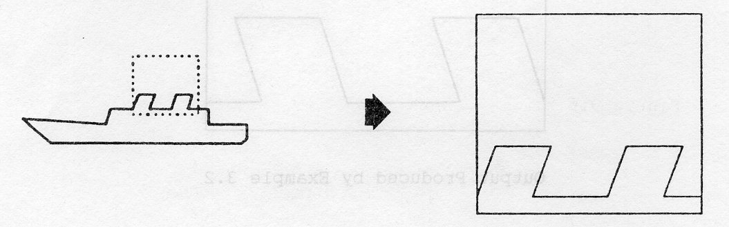
      PROGRAM WV
*                                 GKS Example Program 3.2
*                                 Data for Ship's Outline
      INTEGER NSHIP
      PARAMETER (NSHIP = 18)
      REAL XSHIP(NSHIP), YSHIP(NSHIP)
      DATA XSHIP/0.20,0.10,0.40,0.42,0.50,0.52,0.58,0.56,0.64,
     :          0.66,0.72,0.70,0.78,0.78,0.92,0.92,0.90,0.20/
     :     YSHIP/0.12,0.22,0.20,0.26,0.26,0.32,0.32,0.26,0.26,
     :           0.32,0.32,0.26,0.26,0.20,0.20,0.14,0.12,0.12/
*                                OPEN GKS, OPEN and ACTIVATE WORKSTATION. The
*                                parameters for OPEN GKS and OPEN WORKSTATION
*                                are system- and device- dependent; see Appendix B
*                                for details of the values which are valid on each
*                                system.
      CALL GOPKS (kerrfl, -1)
      CALL GOPWK (1 , kconid, kwtype)
      CALL GACWK (1)
*                                End of standard opening sequence
*----------------------------------------------------------------------------------
*                                Set limits of window surrounding the funnels
      CALL GSWN{1, 50.0,74.0, 24.0,48.0)
      CALL GSELNT(l)
*                                Draw the ship
      CALL GPL(NSHIP,XSHIP,YSHIF)
*----------------------------------------------------------------------------------
*                               Deactivate and close workstation, close GKS
      CALL GDAWK (1)
      CALL GCLWK (1)
      CALL GCLKS
      END
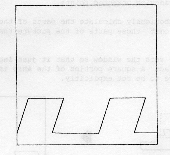
In the example, everything outside the window is removed. It is possible however to specify instead that clipping at the window does not take place. (An additional clip associated with the workstation transformation described later - cannot be turned off). To control whether this happens or not, use SET CLIPPING INDICATOR:
GSCLIP (jclip)
which, according to the value of jclip, sets clipping to be in effect (GCLIP) or not (GNCLIP).
As an example of this, suppose that the same view is mapped to a small viewport. Since we will set the clipping indicator to be GNCLIP (no clipping), we will actually see the whole ship. We add the following calls to the last example:
      CALL GSVP(1, 0.4,0.6, 0.4,0.6)
      CALL GSCLIP(GNCLIP)
producing the following figure.
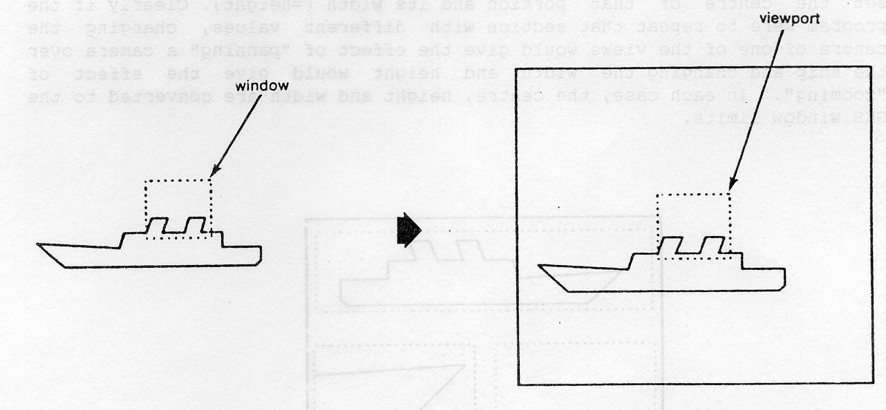
Many graphics programs do not just draw a simple picture with a single coordinate system. For example, there could be a main drawing area with some titles in a margin; or a graph might be drawn in the coordinate system of the data but the tick, marks and the titles may be drawn in some coordinates more akin to the number of squares on graph paper; or different views of the same object might be drawn at different places on the display surface.
In GKS it is possible to set up several coordinate systems by using multiple normalization transformations. For a given normalization transformation, we can specify its window and viewport and, in so doing, are making use of the hitherto artificial integer argument n in SET WINDOW and SET VIEWPORT.
To illustrate this, we shall divide our normalized unit square into 3 views:
To select which portion of the ship is to be viewed in areas 2 and 3, we set the centre of that portion and its width (=height). Clearly if the program were to repeat that section with different values, changing the centre of one of the views would give the effect of panning a camera over the ship and changing the width and height would give the effect of zooming. In each case, the centre, height and width are converted to the GKS window limits.

      PROGRAM MULT
*                                 GKS Example Program 3.3
*                                 (XC2,YC2) is the centre and EXT2 the extent of the
*                                 portion of the ship that is seen in view 2. (XC3,YC3
*                                 and EXT3 have the same role in view 3.
      REAL XC2,YC2, XC3,YC3, EXT2,EXT3, HALF
*                                 Data for Ship's Outline
      INTEGER NSHIP
      PARAMETER (NSHIP = 18)
      REAL XSHIP(NSHIP), YSHIP(NSHIP)
      DATA XSHIP/0.20,0.10,0.40,0.42,0.50,0.52,0.58,0.56,0.64,
     :          0.66,0.72,0.70,0.78,0.78,0.92,0.92,0.90,0.20/
     :     YSHIP/0.12,0.22,0.20,0.26,0.26,0.32,0.32,0.26,0.26,
     :           0.32,0.32,0.26,0.26,0.20,0.20,0.14,0.12,0.12/
*                                OPEN GKS, OPEN and ACTIVATE WORKSTATION. The
*                                parameters for OPEN GKS and OPEN WORKSTATION
*                                are system- and device- dependent; see Appendix B
*                                for details of the values which are valid on each
*                                system.
      CALL GOPKS (kerrfl, -1)
      CALL GOPWK (1 , kconid, kwtype)
      CALL GACWK (1)
*                                End of standard opening sequence
*----------------------------------------------------------------------------------
*                                Set up view 1
      CALL GSWN(1, 0.0,100.0, 10.0,35.0)
      CALL GSVP(1, 0.0,1.0,    0.7,0.95)
*                               Set up view 2 on left of picture
      HALF=EXT2/2.0
      CALL GSWN(2, XC2-HALF,XC2+HALF, YC2-HALF,YC2+HALF)
      CALL GSVP(2,    0.0,   0.5,        0.1,    0.6)
*                               Set up view 3 on right of picture
      HALF=EXT3/2.0
      CALL GSWN(3, XC3-HALF,XC3+HALF, YC3-HALF,YC3+HALF)
      CALL GSVP(3,    0.5,   1.0,        0.1,    0.6)
*                               Now draw the different pieces of ship, by selecting
*                               different views in turn.
      CALL GSELNT(l)
      CALL GPL(NSHIP,XSHIP,YSHIP)
      CALL GSELNT(2)
      CALL GPL(NSHIP,XSHIP,YSHIP)
      CALL GSELNT(3)
      CALL GPL(NSHIP,XSHIP,YSHIP)
*----------------------------------------------------------------------------------
*                               Deactivate and close workstation, close GKS
      CALL GDAWK (1)
      CALL GCLWK (1)
      CALL GCLKS
      END
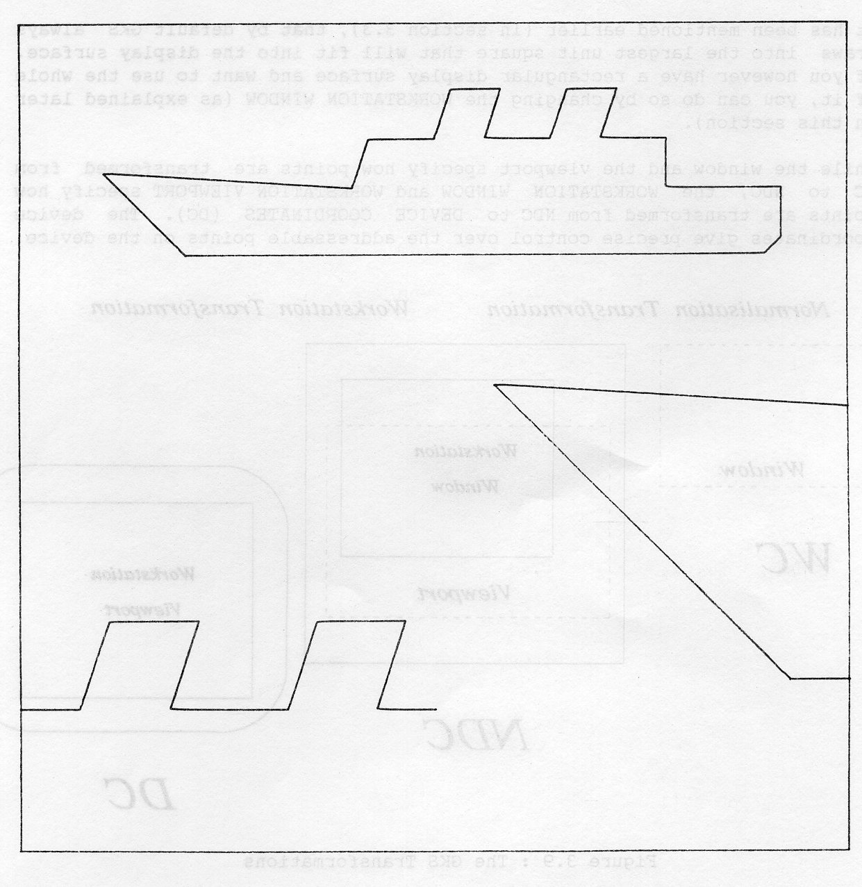
In any GKS implementation, you can set any normalization transformation from 1 to 10. For each the default window is 0 to 1 in both X and Y and also the default viewport. Normalization transformation 0 (which is initially selected for output) is different in that its window and viewport cannot be altered. The examples in chapters 1 and 2 therefore all use normalization transformation 0 by default.
It has been mentioned earlier (in section 3.3), that by default GKS always draws into the largest unit square that will fit into the display surface. If you however have a rectangular display surface and want to use the whole of it, you can do so by changing the WORKSTATION WINDOW (as explained later in this section).
While the window and the viewport specify how points are transformed from WC to NDC, the WORKSTATION WINDOW and WORKSTATION VIEWPORT specify how points are transformed from NDC to DEVICE COORDINATES (DC). The device coordinates give precise control over the addressable points on the device.
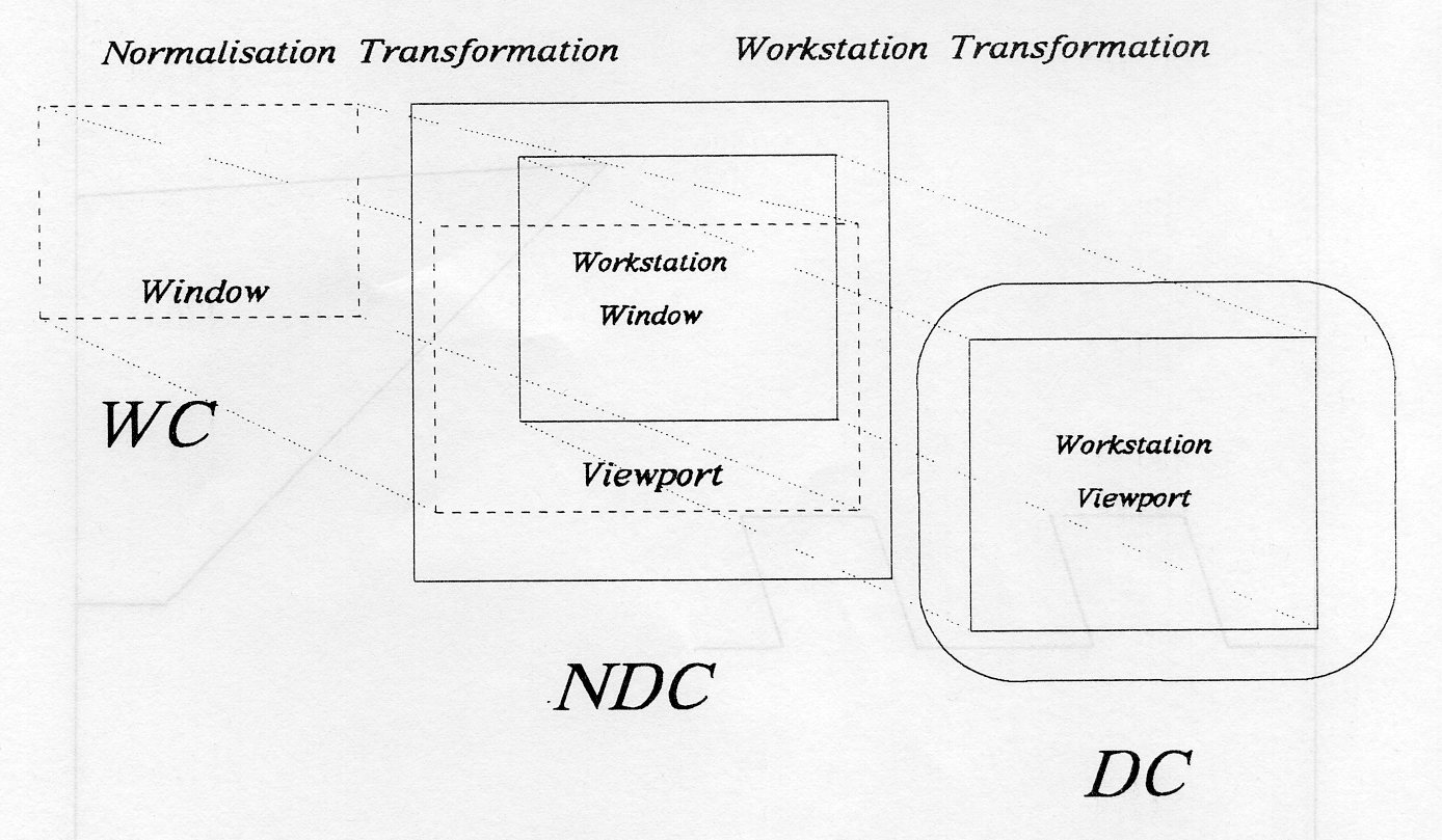
Just as the window specifies the extent of world coordinates that is seen (if the clipping indicator is GCLIP), so the workstation window specifies which portion (default=all) of the NDC unit square is viewed on the display surface. It is set by SET WORKSTATION WINDOW:
GSWKWN (kwkid, xmin, xmax., ymin, ymax)
The workstation identifier kwkid specifies on which open workstation the workstation window is to be set; xmin, xmax, ymin, ymax are all in NDC and together specify the limits of the workstation window, which cannot go outside the NDC unit square.
A small workstation window for example:
CALL GSWKWN(7, 0.4,0.5, 0.2,0.3)
enlarges the picture within it. If a different workstation showed the whole of the NDC unit square:
CALL GSWKWN(8, 0.0,1.0, 0.0,1.0)
then our two workstations would show two different views of the same picture. To fill a whole A4 portrait display surface you use:
CALL GSWKWN(9, 0.0,0.210/0.297, 0.0,1.0)
The workstation viewport specifies which portion of the display surface is to be used and SET WORKSTATION VIEWPORT is used to change it:
GSWKVP (kwkid, xmin, xmax, ymin, ymax)
Again kwkid identifies the open workstation and the other parameters specify the limits of the workstation viewport.
If the workstation window and workstation viewport have different aspect ratios, the shape of the picture within the workstation window is preserved when plotted on the display surface. Circles do not become elongated. To achieve this, the workstation window is always mapped by GKS to the largest portion of the workstation viewport that has the same shape; some of the workstation viewport to the top or to the right might therefore remain unused. Therefore a square workstation window is mapped onto the largest square in the workstation viewport.
By default the workstation window is the NDC unit square and the workstation viewport is the full display surface.
Suppose that the display surface of a particular device is in the ratio 4:3 (wider than it is high). If we allowed the workstation window and workstation viewport to be defaulted, the ship would not use the display to its best advantage. For example, if the viewport were at the bottom of the NDC unit square, thus:
CALL GSVP(1, 0.0,1.0, 0.0,0.25)
the ship would appear as in Figure 3.10. If the workstation window is also made to match the viewport:
CALL GSWKWN(9, 0.0,1.0, 0.0,0.25)
the ship would now use more of the display, as shown in Figure 3.11.
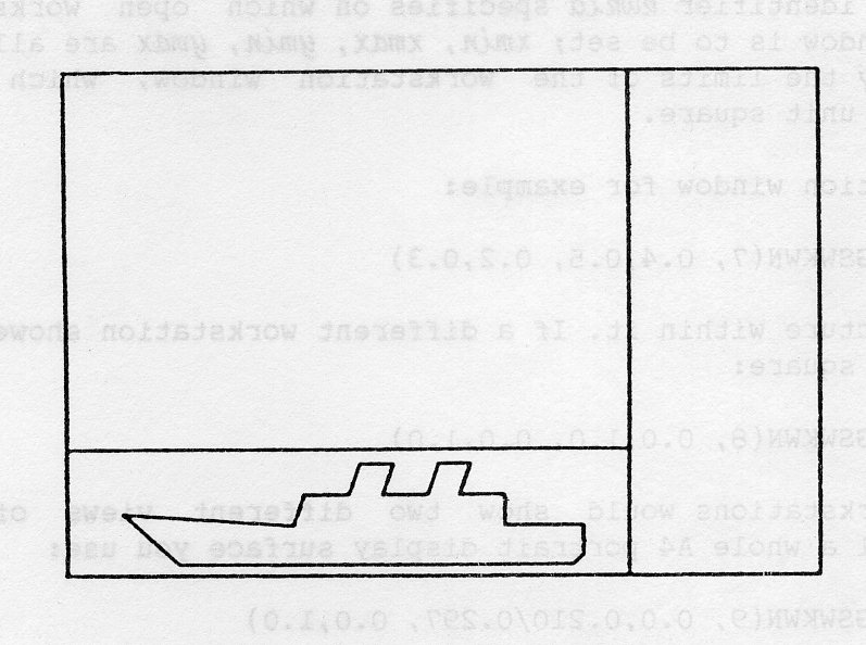

The units of the workstation viewport are device coordinates (DC). For many devices these simply correspond to the addressable units of the display surface or to its raster coordinates. However to ensure that device coordinates can be used in a consistent way, you can assume the following:
which for some devices means that device coordinates do not coincide with the addressable units of the device. For display surfaces on which being able to measure the output is sensible and important (usually plotters), device coordinates are in metres. So on such a device, it is possible to plot within an A4 page as follows:
CALL GSWKVP(7, 0.0,0.210, 0.0,0.297)
(an error occurs if the display surface is not big enough). To use the whole of the A4 page, the workstation window must be shaped to fit:
CALL GSWKWN(7, 0.0,0.210/0.297, 0.0,1.0)
See Section 8.3 for inquiry about the display surface size.
Clipping at the boundary of the workstation window cannot be turned off; the clipping indicator described earlier only applies to the window -> viewport mapping.
The workstation transformation applies to the whole picture. If the workstation window or workstation viewport is altered after some graphics have been drawn, two things are possible:
See Section 8.4.2 for information about window and viewport settings.
In order to use the facilities of GKS, you have to call the OPEN GKS routine:
GOPKS (kerrfl,kbufln)
It takes an error file number kerrfl as a parameter; this is the FORTRAN unit number of the file to be used by GKS for its error messages. You can choose any number within the range of FORTRAN unit numbers allowed on your particular computer/operating system. (See Appendix B for details of this.) The 'file' can also be your terminal. In interactive work, it is useful to route messages to the terminal so that they can be seen immediately. GKS opens a file for the unit if one is not open. The parameter kbufln specifies the amount of memory units required; setting kbufln equal to -1 selects the implementation-dependent default. Note that in RAL GKS, kbufln is ignored.
OPEN GKS may not be called again until you have called CLOSE GKS:
GCLKS
We have already seen how workstations provide the output facilities, and how different workstation types can have different capabilities. So far, all the examples have shown the use of graphical output. GKS provides several categories of workstation, including:
A workstation will often correspond to a physical device, but in some cases a single physical device may support several workstations and in other cases several physical devices may make up a workstation. For example, a screen can contain several output workstations, each in a separate window, and the tablet, keyboard and parts of the screen can form an input workstation.
The set of workstation types available in the RAL GKS library is defined in the Appendix B. You can also find them by calling INQUIRE LIST ELEMENT OF AVAILABLE WORKSTATION TYPES (GQEWK) - see Section 8.2.2.
Before output is sent to a workstation, the workstation has to be opened and activated. When you open a workstation, you pass a workstation identifier, a connection identifier and a workstation type as parameters to
GOPWK (kwkid, kconid, kwtype)
The workstation identifier kwkid is a number that you choose to identify this workstation. You pass this number as a parameter to all workstation-specific routine calls for this workstation (such as INQUIRE POLYLINE REPRESENTATION). The connection identifier kconid allows GKS to connect the workstation with the physical device or devices that support it. The FORTRAN stream numbers that can be used for kconid are system- and device-dependent. Details are given in the binder section Getting Started and in Appendix B.
The workstation type kwtype differentiates between the workstations that are available. Workstation type numbers are listed in Appendix B.
Before output can be sent to a workstation, you must activate it using ACTIVATE WORKSTATION:
GACWK (kwkid)
where kwkid is the workstation identifier. Visible changes can occur on an open but inactive workstation; for example segment attribute changes may cause picture changes (see Chapter 6). Input device simulations may also be drawn on open inactive workstations (see Chapter 5). Workstations which are only used for input cannot be activated. You can have several output workstations active at once - see Appendix B for the limits on each system.
When a workstation is deactivated, using DEACTIVATE WORKSTATION, no further output is sent to it.
GDAWK (kwkid)
You can activate it again, to get more output sent to it.
If a workstation is not active, it can be closed by calling CLOSE WORKSTATION.
GCLWK (kwkid)
You can clear a workstation's display surface by calling CLEAR WORKSTATION.
GCLRWK (kwkid, jclear)
Its second parameter JCLEAR specifies whether the display surface is to be cleared unconditionally (GALWAY), or only if it is not already clear (GCONDI). The use of this parameter is most applicable to plotters, where the effect of clearing the workstation is to move to a new piece of paper.
Not all GKS routines can validly be called at any time. For example, it is not valid to call POLYLINE when no workstation is active. GKS is defined to have five operating states:
Each GKS routine may validly be called in one or more of these operating states. If you call a routine when GKS is in the wrong operating state for that routine, an error message is written to the GKS error file. Although inquiries can be called in any operating state, they return an error indicator if GKS is not in the right operating state for the inquiry to be made.
The MESSAGE routine lets you display a text string on a workstation or on some device associated with it.
GMSG (kwkid, mess)
How it is displayed depends on the workstation.
An example of the use of MESSAGE would be to ask the terminal user to change the paper on a plotter.
An escape function is provided in GKS to allow non-standard action to be taken on appropriate workstations (the use of rasterop hardware, for instance):
GESC (kescid, liesc, iescdn, mloesc, loesc, oescdn)
This routine takes an input array iescdn of liesc CHARACTER*80 strings, which is called the INPUT DATA RECORD. It returns output consisting of loesc CHARACTER*80 strings into an array oescdn of mloesc such strings. This is called the OUTPUT DATA RECORD. If loesc is greater than mloesc, then the OUTPUT DATA RECORD is truncated to mloesc strings.
For instance, an escape that instructs a video or film recorder to repeat each frame of a sequence three times might have function code -201. In this case, the following code would be required:
      CHARACTER*80 DREC(1)
      INTEGER IREC(1)
      IREC(1) = 3
      CALL GPREC(1, IREC, 0, 0.0, 0, ' ', 1, IERR, LDR, DREG)
      CALL GESC(-201, LDR, DREC, 1, LODR, DREG)
The escape functions which are currently supported in RAL GKS are described in Appendix E.
The GKS Fortran 77 language binding defines two utility functions for packing and unpacking data into data records. Data records are used as input and/or output arguments to several GKS routines (e.g. the INITIALISE INPUT routines, ESCAPE, etc.).
The PACK routine is:
GPREC (il, ia, inl, na, isl, lstr, str, mldr, ier, ldr, datrec)
This packs il INTEGERS from array ia, inl REALS from array na and isl CHARACTER strings from CHARACTER array str (with lstr as an array specifying the lengths of each of these strings) into the data record datrec which is a CHARACTER*80 array of dimension mldr. GPREC returns error indicator ier, the data record datrec, and ldr which specifies the number of array elements in datrec which are used.
The unpack routine is the reverse of this:
GUREC (ldr, datrec, idil, idnl, idsl, ier, il, ia, irl, na, isl, lstr, str)
This routine unpacks ldr array elements from the data record CHARACTER*80 array datrec into INTEGER, REAL and CHARACTER arrays ia, na and str (which are dimensioned idil, idnl and isl respectively). ier is the error indicator; il, irl and isl are the number of INTEGER/REAL/CHARACTER string entries, and lstr is an array containing the lengths of the character strings in str.
Many graphical applications want not only to produce output but also to let the user of the application, at a terminal, interact with and modify the output. All computer languages provide a means for programs to get data in from a terminal, at least by supplying data which the user has typed at a keyboard. GKS goes further than this by giving applications a device-independent way of receiving input data from terminals. It does this by defining a set of logical input devices which are associated with a workstation. By describing its input in terms of these logical devices, GKS allows applications to be independent of the physical characteristics of the devices used: many terminals have a way of pointing to a location on the screen, but applications using GKS do not need to know whether a terminal uses a pair of thumbwheels, a mouse, a lightpen or anything else.
The six classes of logical input device in GKS are:
Any workstation which supports input can provide one or more logical input device, although not all workstations may provide all classes of device.
LOCATOR, STROKE and PICK devices return values to the application which are related to a displayed picture. The other classes of device return numerical or character data.
You get input from a device by using a REQUEST routine for that device. Your program is suspended until the input data is available. There is a separate REQUEST routine for each class of logical input device.
The next sections describe the use of device numbers, and then each of the input classes, without going into details about the implementation on particular workstations. This workstation-specific information is given in Appendix C. For each input class the parameters are similar, and in particular the parameters include the workstation identifier, the device number and a status flag. These parameters are described in the section on REQUEST LOCATOR, with additional information given in the sections on REQUEST CHOICE and REQUEST PICK.
On a particular workstation there may be several devices of each class, and you identify each by its number. Device numbers for each class on each workstation are given in Appendix C. Stroke and locator devices are usually closely related to a piece of hardware (such as a pointing device) and there would normally be just one device in each of these classes. Valuator, string and choice devices may have a variety of different representations, and a workstation will often have several of these devices for each class. Every device class has a device number one.
A call to REQUEST LOCATOR returns the coordinates of a position within your picture.
GRQLC (kwkid, klcdnn, jstat, ktnn, xloc, yloc)
You supply the workstation identifier kwkid and the locator device number klcnn. The routine returns a status jstat indicating whether the terminal user has given a locator or used the break action to deny the request. In producing your picture, you may have used several windows and viewports, so as well as the world coordinates xloc and yloc, GKS returns to you the normalization transformation number ktnn that was used to get from the picture displayed on the device to a world coordinate position.
It may be that the chosen position is in more than one viewport, because the viewports in NDC space may overlap. GKS has to choose which viewport (and so which normalization transformation) to use. To allow it to choose, there is a viewport input priority defined for each normalization transformation. The viewport input priority for each normalization transformation is defined simply by its relative position in a sequence. There is no priority number associated with it. Unless you change the priorities, by calling SET VIEWPORT INPUT PRIORITY (GSVPIP), the priorities are in the order of the normalization transformation numbers, with transformation 0 being the highest priority, transformation 1 the next highest and so on. It is important to remember that transformation 0 includes the whole of the NDC space (from 0 to 1 on each axis), and you cannot change transformation 0. This means that unless you change the priorities, you will always get coordinates returned relative to normalization transformation 0.
The following call to SET VIEWPORT INPUT PRIORITY:
GSVPIP (ktnn, kntnn, jrelpn)
moves transformation ktnn so that it is next to transformation kntnn in the priority sequence and is either of higher priority (jrelpn = GHIGHR) or lower priority (jrelpn = GLOWER).
REQUEST STROKE is Similar to REQUEST LOCATOR except that it returns a sequence of points instead of a single point.
GRQSK (kwkid, kskdnn, mp, jstat, ktnn, npoint, xsk, ysk)
Here the parameter mp specifies the maximum number of points that you want to receive (normally the size of your point arrays), and the routine returns the number of points supplied npoint and the arrays of points xsk and ysk. A drawing application might use REQUEST STROKE. A single normalization transformation ktnn is returned, which applies to all the points in the stroke. The set of points may span several viewports, so GKS chooses the viewport with the highest input priority which contains all the points (at least one viewport must contain all the points, as the viewport for normalization transformation 0 contains all points on the display surface).
When the terminal user inputs the set of points, he has to specify each point and also to specify that he has finished the stroke.
Example 5.1 shows the use of viewport input priority and a simple stroke request.
      PROGRAM DRASTR
*                                 GKS Example Program 5.1
*                                 The following variable(s) are defined in the
*                                 include file
*                                 GHIGHR, GNONE
*                                 include GKS parameter file - see Appendix B for details
      INTEGER HP, JSTAT, NPOINT, KSKDNR, KTNR
      PARAMETER (MP=100)
      REAL XSK(MP), YSK(MP)
*                                OPEN GKS, OPEN and ACTIVATE WORKSTATION. The
*                                parameters for OPEN GKS and OPEN WORKSTATION
*                                are system- and device- dependent; see Appendix B
*                                for details of the values which are valid on each
*                                system.
      CALL GOPKS (kerrfl, -1)
      CALL GOPWK (1 , kconid, kwtype)
      CALL GACWK (1)
*                                End of standard opening sequence
*----------------------------------------------------------------------------------
      KSKDNR = 1
*                                Set up a window, and viewport input priority
      CALL GSWN (1, 0.0, 100.0, 0.0, 100.0)
      CALL GSELNT (1)
      CALL GSVPIP (1, 0, GHIGHR)
*                                Input the stroke
      CALL GRQSK (1, KSKDNR, HP, JSTAT, KTNR, NPOINT, XSK, YSK)
*                                Number of points is in NPOINT.  Mark each point.
      IF (JSTAT .NE. GNONE) CALL GPM (NPOINT, XSK, YSK)
*----------------------------------------------------------------------------------
*                               Deactivate and close workstation, close GKS
      CALL GDAWK (1)
      CALL GCLWK (1)
      CALL GCLKS
      END
A call to REQUEST VALUATOR returns a real number.
GRQVL (kwkid, kvldnn, jstat, val)
The real number is in val. The way in which GKS allows the terminal user to specify a real number depends on the facilities available on the particular device.
REQUEST CHOICE returns an integer representing the number of the choice that has been made.
GRQCH (kwkid, kchdnn, jstat, kchnn)
You may have displayed a number of options for the terminal user to choose from, or you may want the options to be displayed as part of the choice request. REQUEST CHOICE allows both the simple choice option (the terminal user might press a key on the keyboard) and more complex cases where a set of strings is displayed for the duration of the choice request. The choice number is returned in kchnn. The status is returned in jjstat, indicating whether the terminal user has given a choice (jstat = GOK), made no choice (jstat = GNCHOI) or used the break action to deny the request (jstat = GNONE).
A pick device allows the terminal user to select part of a picture by pointing to it. When you use REQUEST PICK, the program is suspended until you identify a point in the displayed picture using an input device.
GRQPK (kwkid, kpkdnn, jstat, ksegnm, kpkid)
The pick device number is kpkdnn. The status jstat indicates, if no part of the picture has been identified (jstat = GNPICK), some part of the picture has been identified (jstat = GOK) or the break action has been invoked (jstat = GNONE). The name of the segment identified by the pick device is ksegnm and the pick identifier of the part selected is kpkid. (For a description of segments see Chapter 6, and Section 6.7 for pick identifiers).
REQUEST STRING returns a character string.
GRQST (kwkid, kstdnn, jstat, lstr, str)
The length of the string is returned in lstr, and the string in str. On most devices the string would be input by the user typing at a keyboard.
For each device class, there is an INITIALISE routine which allows some specific features of the device representation to be selected. You do not have to initialise a device, as all devices have default values set.
If you want to write programs that can be used without change on a variety of hardware devices, or that are easily portable to other implementations of GKS, it will be easier if you do not use the initialise features (which, apart from the initial values, tend to be device-specific). On the other hand, it is only by using the INITIALISE routines that you will be able to take advantage of the full facilities of particular devices.
If a logical device does not exist in hardware, it may be presented as a simulation on the display surface. For example, valuator devices may be drawn to represent potentiometers, and allow selection of a value by pointing to a position on the drawn simulation. The position of this simulated device on the display surface is called the echo area.
A device of this sort has a default echo area, but you can change this by specifying your own echo area by parameters to the INITIALISE routines. Some device types do not need an echo area (this will often be the case for locator devices).
Input from devices is obtained in various ways, depending on the current mode of the device. Each logical input device can be operated in one of three modes - REQUEST, SAMPLE or EVENT. GKS provides a number of functions of the form SET XXX MODE, where XXX is one of LOCATOR, STROKE, CHOICE, VALUATOR, PICK or STRING. These functions are used to specify the operating mode of a particular device and to switch echoing on and off.
The only operating mode supported at GKS implementation level 2b is REQUEST mode, so these routines are used only to switch echoing on and off. For LOCATOR this is
GSLCM (kwkid, klcdnn, jmode, jesw)
where kwkid is the workstation identifier, klcdnn the locator device number, jmode. the operating mode (always REQUEST at this level of GKS) and jesw is the ECHO SWITCH that specifies whether echoing is on (jesw = GECHO) or off (jesw = GNECHO).
The way in which a logical device is presented to the terminal user is determined by the Prompt and Echo Type (PET) which you have selected for that device. The prompt is the way in which the terminal user is prompted to supply input (often by something being displayed to catch his attention) and the echo is the way in which the system gives him feedback while he is doing the interaction. For example, on a locator device the prompt would normally be the display of a special cursor shape, and the echo would be the way in which the displayed cursor moved about the screen in response to the user's actions, by moving a pointing device, mouse or thumbwheels.
For each device number within a class, there may be a choice of several PETs. They are all listed in Appendix C. On a locator device, for example, the PETs may be:
and so on.
Each class of device lets you specify some initial values which are used when the device is first displayed. For each input class, there is an initialisation function which can only be used if the input device is in REQUEST MODE. These initialisation functions have the form INITIALISE XXX, where XXX is one of LOCATOR, STROKE, CHOICE, VALUATOR, PICK or STRING.
An application program can use the appropriate initialisation function to adjust the measure of an input device to some sensible or expected value; the terminal user then needs only to confirm that value or change it to some other (hopefully close value). For example, the function INITIALISE LOCATOR may be used to specify the initial position of the cursor on the screen to be close to where the device is expected to be triggered. This minimises the average distance that the cursor needs to be moved before the device is actually triggered.
GINLC    (kwkid, klcdnn, ktnn, xinloc, yinloc, kpet, xmin, xmax,
          ymin, ymax, minprd, inpdn)
The workstation identifier is kwkid, the locator device number isklcdnn and the initial normalisation transformation number is ktnn. The initial locator position is given by (xinloc,yinloc). The prompt and echo type is specified by kpet. The bounds of the echo area are given by xmin left, xmax right, ymin bottom and ymax top. If any additional information about a locator device has to be supplied to the initialisation function, it is passed via a data record inpdn, which is an array of minpdn character*80 elements. The INITIALISE functions for other input classes have similar arguments and are of the form GINxx, where xx is one of (SK, CH, VL, PK, ST).
The GKS output facilities let you draw pictures, but do not let you move completed pictures or parts of pictures. GKS segments give you the ability to produce a picture in the normal way and then modify parts of it, for example by moving the parts around.
An application program can split its picture into a number of segments. Each segment consists of a set of output primitives, and has some segment attributes which can be modified to alter the appearance of the segment.
To get output stored in a segment, you must create a segment. This segment is known as the open segment. Only one segment can be open at a time, and all output is stored in the segment as well as being sent to all active workstations. The open segment can be closed and another segment created; each segment is identified by a name, which is a positive integer. Segments can be renamed, but not reopened: once a segment has been closed, no further output can be added to that segment.
A segment has a set of attributes associated with it, including a segment transformation, which lets you move the segment around. This transformation is applied after the normalization transformation. The identity transformation is used as the segment transformation until you set another transformation.
Segments can be deleted from a particular workstation, or from all workstations.
You create a segment using CREATE SEGMENT:
GCRSG (ksegnm)
giving it an integer name ksegnm by which the segment is known. This name must be different from all other segments' names. When a segment has been created, it becomes the open segment and all output primitives are stored in the segment. Only one segment can be open at a time, so a call to CREATE SEGMENT will fail if you issue it before you have closed a previously created segment.
When you have finished outputting to a segment, you call CLOSE SEGMENT.
GCLSG
Example 6.1 shows the use of CREATE SEGMENT and CLOSE SEGMENT. The output primitives are sent to the active workstation and stored in the segment. All the attributes associated with the output primitives are also stored in the segment; the importance of this will become clear in later examples of the use of segment attributes.
      PROGRAM SEG1
*                                 GKS Example Program 6.1
*                                 Data for Ship's Outline
      INTEGER NSHIP
      PARAMETER (NSHIP = 18)
      REAL XSHIP(NSHIP), YSHIP(NSHIP)
      DATA XSHIP/0.20,0.10,0.40,0.42,0.50,0.52,0.58,0.56,0.64,
     :          0.66,0.72,0.70,0.78,0.78,0.92,0.92,0.90,0.20/
     :     YSHIP/0.12,0.22,0.20,0.26,0.26,0.32,0.32,0.26,0.26,
     :           0.32,0.32,0.26,0.26,0.20,0.20,0.14,0.12,0.12/
*                                OPEN GKS, OPEN and ACTIVATE WORKSTATION. The
*                                parameters for OPEN GKS and OPEN WORKSTATION
*                                are system- and device- dependent; see Appendix B
*                                for details of the values which are valid on each
*                                system.
      CALL GOPKS (kerrfl, -1)
      CALL GOPWK (1 , kconid, kwtype)
      CALL GACWK (1)
*                                End of standard opening sequence
*----------------------------------------------------------------------------------
*                                Create segment number 1
      CALL GCRSG (1)
*                                Now output to it
      CALL GSPLI (2)
      CALL GPL (NSHIP, XSHIP, YSHIP)
*                                Close the segment
      CALL GCLSG
*----------------------------------------------------------------------------------
*                               Deactivate and close workstation, close GKS
      CALL GDAWK (1)
      CALL GCLWK (1)
      CALL GCLKS
      END
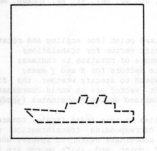
The representation of a picture is affected by the attributes which are applied to the output primitives (for example, linestyle) and by the transformations which are applied to take them from your world coordinates to the device coordinates for each device on which they are displayed. When output primitives are grouped into a segment, there are attributes associated with the segment which can be used as a further modification of the picture representation. These attributes are described in the next subsections.
Each segment has associated with it a transformation which is applied to all the output primitives in the segment after the normalization transformation has been applied. This transformation lets you scale, rotate and shift the segment. Until you change it, each segment transformation is set to the identity transformation, which means that only the usual transformations from world coordinates to NDC and DC are applied. You can change a segment transformation at any time, for closed segments or the open segment. The GKS routine is SET SEGMENT TRANSFORMATION.
GSSGT (ksegnm,segtrn)
The effect of changing a transformation applies at once (although you can defer the change: this is covered later in the chapter), and the way that the change is shown depends on the type of device. More details are given below.
A segment transformation segtrn, is defined as a 2x3 transformation matrix. It is not very easy to construct this matrix, so GKS provides two utility routines to make it easier. These routines are EVALUATE TRANSFORMATION MATRIX and ACCUMULATE TRANSFORMATION MATRIX.
GEVTM (xo, yo, dx, dy, phi, fx, fy, jcotyp, matout)
The parameters are:
            xo,yo: a fixed point (for scaling and rotation);
dx,dy: a shift vector for translation;
phi:   an angle of rotation in radians;
fx,fy: scale factors for x and y axes;
jcotyp:a switch to specify whether the fixed point and the
                shift vector are in world coordinates (jcotype = GWC) or
                normalized device coordinates (jcotyp = GNDC)
The transformation applies in this order (scale, rotate, shift), and the routine returns the corresponding transformation matrix in matout. You would normally set the coordinate switch to specify world coordinates. In this case, the fixed point and shift vector are transformed using the current normalization transformation. Example 6.2 uses EVALUATE TRANSFORMATION MATRIX to produce a transformation matrix which decreases the size of the ship to half its original size, rotates it through 15 degrees anticlockwise (pi/12 radians) and shifts it by 0.2 in the X direction. Figure 6.1 shows the three stages of scale, rotation and shift which are performed (always in that order) to give the final picture. In this example, the transformation is changed after the ship has been output, so the ship will appear to move. If you wanted to draw the ship initially in the transformed position, you would change the transformation before drawing the ship.
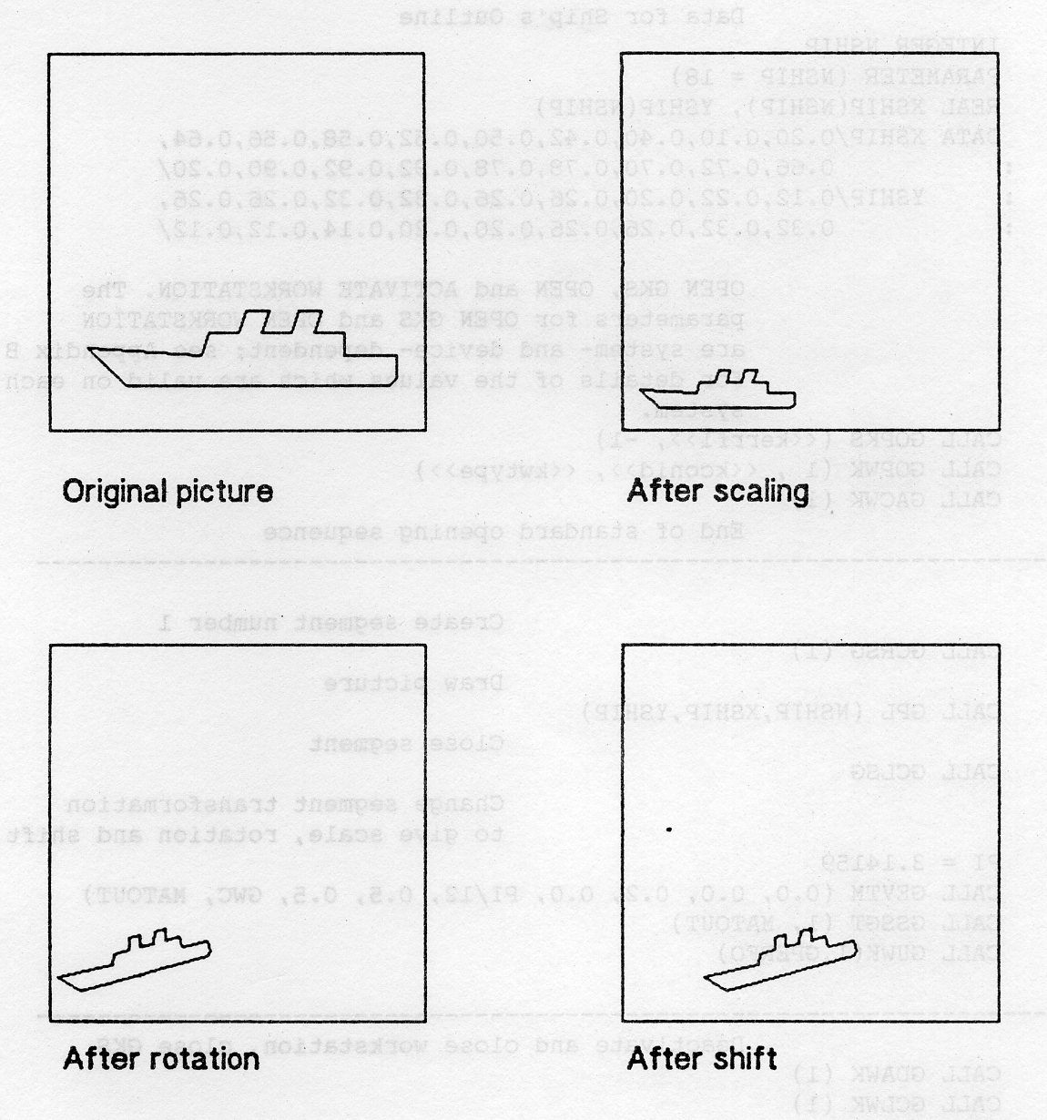
      PROGRAM SEG2
*                                 GKS Example Program 6.2
*                                 The following variable(s) are defined in the
*                                 include file
*                                 GWC, GPERFO
*                                 include GKS parameter file - see Appendix B for details
      REAL MATOUT (2,3)
      REAL PI
*                                 Data for Ship's Outline
      INTEGER NSHIP
      PARAMETER (NSHIP = 18)
      REAL XSHIP(NSHIP), YSHIP(NSHIP)
      DATA XSHIP/0.20,0.10,0.40,0.42,0.50,0.52,0.58,0.56,0.64,
     :          0.66,0.72,0.70,0.78,0.78,0.92,0.92,0.90,0.20/
     :     YSHIP/0.12,0.22,0.20,0.26,0.26,0.32,0.32,0.26,0.26,
     :           0.32,0.32,0.26,0.26,0.20,0.20,0.14,0.12,0.12/
*                                OPEN GKS, OPEN and ACTIVATE WORKSTATION. The
*                                parameters for OPEN GKS and OPEN WORKSTATION
*                                are system- and device- dependent; see Appendix B
*                                for details of the values which are valid on each
*                                system.
      CALL GOPKS (kerrfl, -1)
      CALL GOPWK (1 , kconid, kwtype)
      CALL GACWK (1)
*                                End of standard opening sequence
*----------------------------------------------------------------------------------
*                                Create segment number 1
      CALL GCRSG (1)
*                                Draw picture
      CALL GSPLI (2)
      CALL GPL (NSHIP, XSHIP, YSHIP)
*                                Close the segment
      CALL GCLSG
*                                Change segment transformation
*                                to give scale, rotation and shift
      PI = 3.14159
      CALL GEVTM (0.0, 0.0, 0.2, 0.0, PI/12, 0.5, 0.5, GWC, MATOUT)
      CALL GSSGT (1, MATOUT)
      CALL GUWK(1,GPERFO)
*----------------------------------------------------------------------------------
*                               Deactivate and close workstation, close GKS
      CALL GDAWK (1)
      CALL GCLWK (1)
      CALL GCLKS
      END
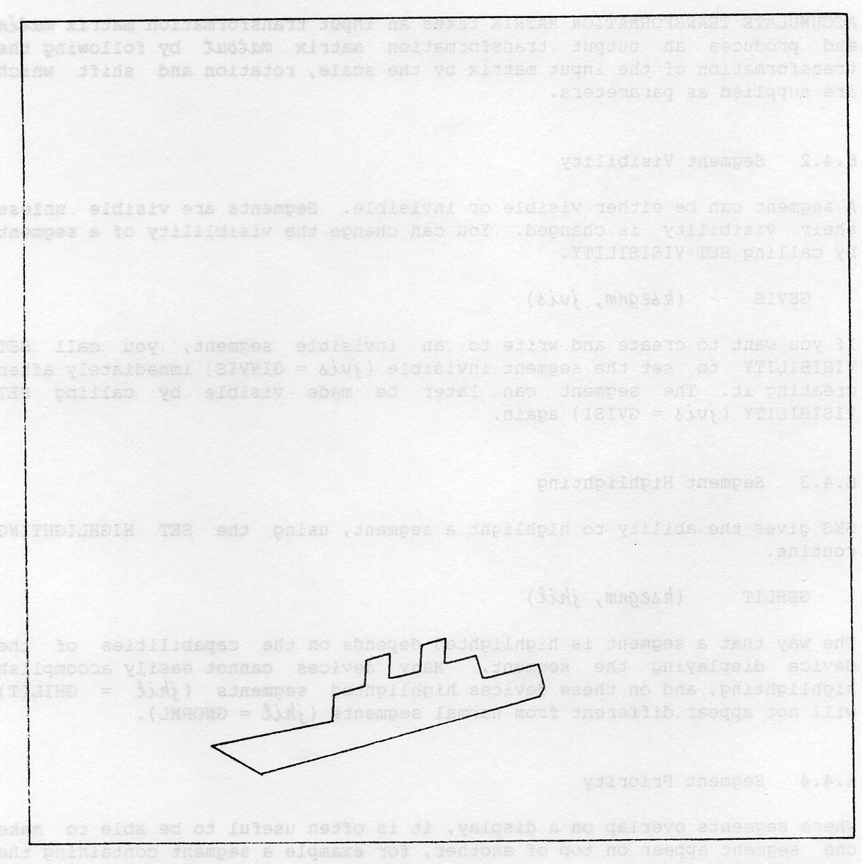
If you wanted to do the shift before the rotation, you could use EVALUATE TRANSFORMATION MATRIX to produce a matrix which does the scale and shift, with no rotation, and then call ACCUMULATE TRANSFORMATION MATRIX to add the rotation.
GACTM (mtfa, xo, yo, dx, dy, phi, fx, fy, jcotyp, matout)
ACCUMULATE TRANSFORMATION MATRIX takes an input transformation matrix and produces an output transformation matrix matout by following the transformation of the input matrix by the scale, rotation and shift which are supplied as parameters.
A segment can be either visible or invisible. Segments are visible unless their visibility is changed. You can change the visibility of a segment by calling SET VISIBILITY.
GSVIS (ksegnm, jvis)
If you want to create and write to an invisible segment, you call SET VISIBILITY to set the segment invisible (jvis = GINVIS) immediately after creating it. The segment can later be made visible by calling SET VISIBILITY ((jvis = GVISI) again.
GKS gives the ability to highlight a segment, using the routine SET HIGHLIGHTING.
GSHLIT (ksegnm, jhil)
The way that a segment is highlighted depends on the capabilities of the device displaying the segment. Many devices cannot easily accomplish highlighting, and on these devices highlighted segments (jhil = GHILIT) will not appear different from normal segments (jhil = GNORML).
Where segments overlap on a display, it is often useful to be able to make one segment appear on top of another, for example a segment containing the background of a picture should appear behind a segment containing the foreground of the picture. You can use SET SEGMENT PRIORITY to control this:
GSSGP (ksegnm, prior)
Each segment can be given a priority prior in the range 0 to 1, where 0 is the lowest priority. If a display device cannot fully support segment priorities, then this implementation of GKS can give limited support within the GKS software which controls the device: segment priority is only taken into account when a complete regeneration of the picture is done, and apart from this segments are drawn on top of the current picture. For some devices, such as pen plotters, no support for segment priorities can be given. You can make sure that your picture is correct by calling the routine REDRAW ALL SEGMENTS ON WORKSTATION.
Any drawing done outside a segment takes no account of segment priority; it goes on top of anything already displayed.
A segment can be deleted from a specific workstation, or deleted completely. The routine DELETE SEGMENT FROM WORKSTATION causes the segment to disappear from the display surface of the specified workstation.
GDSGWK (kwkid, ksegnm)
DELETE SEGMENT causes the segment to disappear from all workstations, and then you can use the segment name again in a subsequent CREATE SEGMENT call.
GDSG (ksegnm)
You can delete all the segments from a workstation by calling CLEAR WORKSTATION.
You can rename a segment, whether open or closed, by calling RENAME SEGMENT.
GRENSG (namold, namnew)
namold and namnew are the old and new segment names.
Section 5.7 described REQUEST PICK, which allows the terminal user to select part of a picture. When REQUEST PICK is called, the program is suspended until the terminal user identifies by means of an input device, a point in the displayed picture. REQUEST PICK then returns the name of the segment containing the point and an identifier, which further identifies part of the picture within the segment. The following sections describe how to ensure the point selected correctly identifies the required part of the picture.
If a segment is created for each identifiable part of the picture, then the returned segment name uniquely identifies the required drawing. However this would be very inefficient (on segment store) if this were done for a large number of identifiable parts. In such a case, it is probably better to use PICK IDENTIFIERS to identify picture components in each segment.
You use SET PICK IDENTIFIER to specify and identifier to do this.
GSPKID (kpkid)
kpkid is an integer value, used as the pick identifier.
Subsequent drawings performed by the output primitives will be associated with this identifier, until a further call to GSPKID is made to indicate that drawing for this picture component is complete and a new component is to be started.
When REQUEST PICK is used and a component associated with a pick identifier is selected, it returns that pick identifier along with the segment name. If no pick identifier has been specified, REQUEST PICK returns the default pick identifier, which is 0.
You can control the information returned by pick by making a segment DETECTABLE so that it can be identified by a pick input device or UNDETECTABLE so that it cannot.
Suppose for example, there are two overlapping segments, one representing the background of a picture and the other an object in the foreground. Suppose also that the foreground object is one of a set of objects that you want to be able to select. A point that is within this foreground object is also within both of these segments, but it the foreground object whose segment name and pick identifier you want to be returned. You can ensure this by making the background segment undetectable and the foreground one detectable.
By default, all segments are undetectable, so you must make a segment detectable if you want to offer it for selection. You can use SET DETECTABILITY to alter this detectability attribute for a named segment.
GSDTEC (ksegnm, jdet)
jsegnm is the name of the segment whose detectability is to be changed and jdet is an integer which specifies whether the segment is to be made detectable (jdet = GDETEC) or undetectable (jdet = GUNDET).
Note: REQUEST PICK returns a status value jstat which is GOK if the requested information has been provided, GNPICK if a point not in a detectable segment has been selected and GNONE is a break action has occurred.
If the point selected by the device lies in two or more detectable segments, then the defined segment priorities determine which segment name is returned.
The appearance of a segment is unchanged, when its detectability is changed. If its segment is invisible, it will not be selected by a PICK input device, regardless of detectability.
When you change a segment transformation, make a segment invisible, or delete a segment, the visual effect depends on the workstation, and on the setting of the implicit regeneration mode (see below). On some workstations, segments can be modified without affecting the rest of the picture. On pen plotters, a segment can only be modified by redrawing the whole picture. On many raster workstations, it may be possible to modify a segment, but in a way which leaves traces of the segment on the rest of the picture (consider a segment which consists of a red line, and it has been drawn across a yellow filled area: the workstation may choose to erase the line by drawing it in the background colour, leaving a black line across the yellow area instead of a red line). In such a case, GKS will be aware that the picture may not be perfect, and will set a flag to indicate that the picture needs updating. You can control the visual effects of segment deletion by using the implicit regeneration mode.
Each workstation has a deferral mode which allows you to control the way in which output is sent to the workstation. Applications will usually want their output to be displayed on a workstation as soon as possible, but there are some circumstances when it may be better to delay the output. These circumstances might be when a workstation's display surface is on a networked terminal which is connected to the host computer. In this case, to send each output request to the terminal as it occurs may be less efficient than allowing output requests to be stored in a buffer until it is full and then sent. If you are prepared to allow output to be deferred in this way, you can call SET DEFERRAL STATE to set the deferral mode to one of the following values.
A workstation may choose not to defer output, but to output immediately.
Each workstation also has an implicit regeneration mode. Many GKS routines are able to produce their output without affecting the rest of the picture, but in some cases the effect of a GKS routine on a workstation may mean that the whole picture has to be regenerated in order to get the picture displayed properly. One example of this was given above, in the section on visible effects of segment routines. Another example is SET COLOUR REPRESENTATION: on raster displays, a change to the colour representation can usually be achieved without regenerating the picture, but on a pen plotter a new picture would have to be drawn.
Regenerating the whole picture may take a long time, so you may want to continue with the current picture, even though it is not a perfect representation, and only regenerate the whole picture later. For any picture change on a workstation, GKS knows whether the effect has made a picture regeneration necessary, and it will take action depending on the setting of the implicit regeneration mode. You can set this to one of two values:
SET DEFERRAL STATE lets you set the implicit regeneration mode jregmo as well as the deferral mode jdefmo.
GSDS (kwkid, jdefmo, jregmo)
The sections above explain how a picture on a workstation can be out of date. You can make sure that the picture is completely up to date by calling UPDATE WORKSTATION or REDRAW ALL SEGMENTS ON WORKSTATION. Whenever the picture is regenerated, all output primitives which are not held in segments are lost; the complete picture consists only of the segments which have been stored on the workstation. The output primitives are stored in segments together with the attributes which applied when they were drawn. When a picture is redrawn, these same attributes are applied to the output primitives, regardless of changes to the attributes which may have taken place after the primitive was stored in the segment. This means, for example, that a polyline that was stored in a segment when the current linetype was dotted will be output as a dotted polyline when the picture is regenerated even if the current linetype has changed to dashed.
UPDATE WORKSTATION ensures that the workstation's picture is completely up to date.
GUWK (kwkid, jregfl)
The parameter jregfl lets you specify whether the picture may be regenerated (GPERFO, perform) or not (GPOSTP, postpone). If you specify GPERFO, it may be necessary to regenerate the whole picture but if it is not necessary it will not be done. This means that primitives which were not stored in a segment may or may not still be in the picture after the update.
As this implementation gives only limited support to segment priority, GKS may think that the picture is up to date even though segments are displayed in the wrong priority order. If you need the segments displayed with the correct priorities, you should call REDRAW ALL SEGMENTS ON WORKSTATION.
REDRAW ALL SEGMENTS ON WORKSTATION brings the picture up to date executing any deferred actions and then regenerates the whole picture.
GRSGWK (kwkid)
In Example 6.3, a picture is composed in three segments: two ships and a horizon, with some stars drawn outside a segment. Although the ships are displayed in the wrong priority order, GKS does not regenerate the picture when UPDATE WORKSTATION is called because the update regeneration flag is set to GPOSTP (postpone). When REDRAW ALL SEGMENTS ON WORKSTATION is called, however, the picture is redrawn with the segments in the right order.
      PROGRAM SEGPRI
*                                 GKS Example Program 6.3
*                                 The following variable(s) are defined in the
*                                 include file
*                                 GPOSTP, GPATTR, GWC
*                                 include GKS parameter file - see Appendix B for details
      REAL MATOUT(2,3),HORX(6),HORY{6),STARX(10),STARY(10)
      INTEGER JASF{13)
      REAL PI
*                                 Data for Ship's Outline
      INTEGER NSHIP
      PARAMETER (NSHIP = 18)
      REAL XSHIP(NSHIP), YSHIP(NSHIP)
      DATA XSHIP/0.20,0.10,0.40,0.42,0.50,0.52,0.58,0.56,0.64,
     :          0.66,0.72,0.70,0.78,0.78,0.92,0.92,0.90,0.20/
     :     YSHIP/0.12,0.22,0.20,0.26,0.26,0.32,0.32,0.26,0.26,
     :           0.32,0.32,0.26,0.26,0.20,0.20,0.14,0.12,0.12/
      DATA HORX/0.0, 0-2, 0.4, 0.6, 0.8, 1.0/
      DATA HORY/0.56, 0.56, 0.54, 0.56, 0.54, 0.55/
      DATA STARX/0.1, 0.2, 0.3, 0.4, 0.5, 0.6, 0.7, 0.8, 0.9, 0.55/
      DATA STARY/0.7, 0.65, 0.92, 0.68, 0.84, 0.77, 0.86, 0.95,
     :           0.62, 0.66/
      DATA JASF/0,0,0,1,0,0,0,0,0,0,1,1,0/
*                                OPEN GKS, OPEN and ACTIVATE WORKSTATION. The
*                                parameters for OPEN GKS and OPEN WORKSTATION
*                                are system- and device- dependent; see Appendix B
*                                for details of the values which are valid on each
*                                system.
      CALL GOPKS (kerrfl, -1)
      CALL GOPWK (1 , kconid, kwtype)
      CALL GACWK (1)
*                                End of standard opening sequence
*----------------------------------------------------------------------------------
*                                Set ASFs for individual patterns and markers
      CALL GSASF (JASF)
*                                Set fill area style patterned
      CALL GSFAIS (GPATTR)
*                                Draw ship in segment l
      CALL GCRSG (1)
      CALL GSFASI (1)
      CALL GFA (NSHIP, XSHIP, YSHIP)
      CALL GCLSG
*                                Draw a smaller ship in segment 2
      CALL GCRSG (2)
      CALL GEVTM (0.0, 0,0, 0.4, 0.2, 0.0, 0.4, 0.6, GWC, MATOUT)
      CALL GSSGT (2, MATOUT)
      CALL GSFASI (2)
      CALL GFA (NSHIP, XSHIP, YSHIP)
      CALL GCLSG
*                                Draw horizon in segment 3
      CALL GCRSG (3)
      CALL GPL (6, HORX, HORY)
      CALL GCLSG
*                                Draw some stars outside a segment
      CALL GSMK (3)
      CALL GPM (10, STAPX, STARY)
*                                Set segment priorities 1>2>3
      CALL GSSGP (1, 0.8)
      CALL GSSGP (2, 0.6)
      CALL GSSGP (3, 0.1)
*                                Update workstation: postpone
      CALL GUWK (1, GPOSTP)
*                                Redraw all segments in priority order (stars go)
      CALL GRSGWK (1)
*----------------------------------------------------------------------------------
*                               Deactivate and close workstation, close GKS
      CALL GDAWK (1)
      CALL GCLWK (1)
      CALL GCLKS
      END
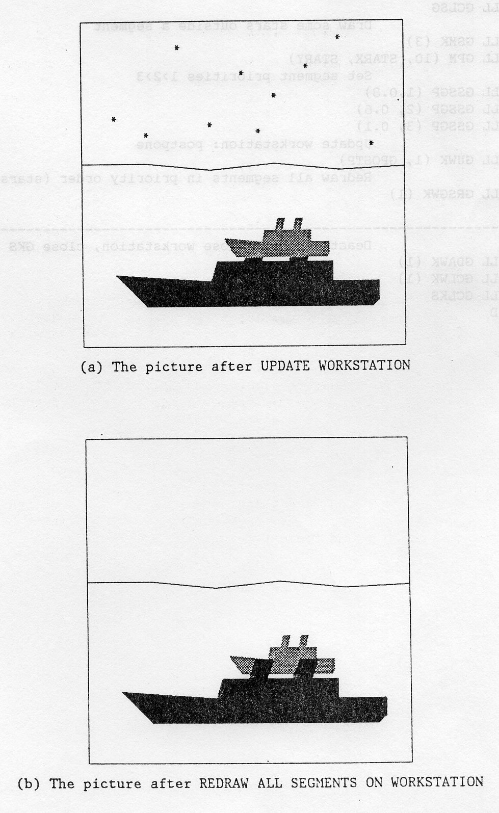
Until now, this Chapter has described how parts of drawings can be manipulated by naming them as segments which exist on all workstations which are active when the segments are created. You can also create segments which are independent of any workstation; this facility is known as Workstation Independent Segment Storage (WISS). The use of WISS in conjunction with segments which are linked to workstations provides more powerful facilities for picture manipulation. For example, WISS makes it easier for you to develop your picture on a screen display and produce a hard copy on a plotter when the picture is fully developed. WISS can also He useful if you want to show identical features in different parts of your picture.
WISS facilities are made available by considering WISS to be a special type of workstation which, like any other workstation, is identified by a workstation type number. The WISS workstation must be opened and activated in exactly the same way as any other workstation. If the WISS workstation is active when a segment is created, then the segment exists in WISS as well as on any other workstations which are active at that time. The segment functions described in Section 6.4 operate on WISS segments just as they do on segments created on other workstations. There are also three special WISS segment functions which allow you to transfer drawings from WISS to other workstations; these are described in the following sections.
Suppose that you want to compose the background of a picture on an interactive workstation, and then want to reproduce the final composition many times on a plotter. (For example, this technique is useful if you are creating a cartoon, where the background remains constant over a number of successive frames.) You can use the routine ASSOCIATE SEGMENT WITH WORKSTATION to do this.
You start by activating a workstation with a screen display surface, together with the WISS workstation. When you are satisfied with the image, you can use ASSOCIATE SEGMENT WITH WORKSTATION to copy the segment from WISS to a plotter; following this, the segment also exists on the plotting workstation, and will appear on every frame produced on the plotter until the segment is changed in some way. (The standard segment functions operate on this workstation in the same way as the others.)
GASGWK (kwkid, ksegnm)
kwkidspecifies the workstation identifier for the workstation to which the segment is to be copied, and ksegnm specifies the name of the segment to be copied. Note that ASSOCIATE SEGMENT WORK WORKSTATION cannot be used if there is currently an open segment.
COPY SEGMENT TO WORKSTATION copies the image stored in a named segment from the WISS workstation to another named workstation. This routine differs from ASSOCIATE SEGMENT WITH WORKSTATION in that, although the picture is transferred so that the immediate visual effect is the same, the picture does NOT exist as a segment on the workstation to which it is transferred, and is therefore unaffected by further segment manipulation; it is as if the output primitives used to compose the picture in the segment had been called directly.
You can use COPY SEGMENT TO WORKSTATION to copy identical parts of a picture to different positions. This may be achieved by ensuring that the WISS workstation is active when the segment is created, and then applying a segment transformation to manipulate the segment to the first position; the segment can then be copied in this position. A further segment transformation can then be applied to move the segment to a new position where it can again be copied, and so on. Note that you could also use COPY SEGMENT TO WORKSTATION with ASSOCIATE SEGMENT WITH WORKSTATION to put a picture on a standard background.
GCSGWK (kwkid, ksegnm)
kwkid specifies the workstation identifier for the workstation to which the segment is to be copied, and ksegnm specifies the name of the segment to be copied. Note that COPY SEGMENT TO WORKSTATION cannot be used if there is currently an open segment.
INSERT SEGMENT copies the picture in a named segment in the WISS workstation to all active workstations; it also allows you to specify a transformation matrix to be applied before the picture is displayed on these workstations.
INSERT SEGMENT differs from ASSOCIATE SEGMENT WITH WORKSTATION and COPY SEGMENT TO WORKSTATION in that it can be used when a segment is open. If there is an open segment, the copied drawing becomes part of the drawing for that segment on all active workstations (the WISS workstation may be one of these). If there is no open segment, the picture is copied to all active workstations, but does not form part of any segment on these workstations.
GINSG (ksegnm, segtrn)
ksegnm specifies the name of the segment in WISS containing the picture element to be copied, and segtrn is the name of a real array holding the transformation matrix for the transformation to be applied. The specified transformation is applied after any transformation specified for the segment by SET SEGMENT TRANSFORMATION. INSERT SEGMENT also differs from the other WISS segment functions in that it is possible to change the rectangle at which clipping is applied. Section 3.5 explained how window and viewport settings may be used to eliminate unwanted parts of a picture by clipping at the viewport boundary. When a picture is created as a segment, it is transformed using the currently selected normalization transformation before being stored as a segment. The segment is thus defined using normalized device coordinates, and the displayed picture is clipped at the boundary of the viewport used for the normalization transformation. However, if you are using INSERT SEGMENT, then although the segment has already been transformed to normalized device coordinates using the transformation which was current when the segment was created, clipping is applied at the boundary of the viewport for the transformation selected when INSERT SEGMENT is used. Example 6.4 illustrates how WISS can be used.
      PROGRAM WISS
*                                 GKS Example Program 6.4
      REAL MATRX1(2,3), MATRX2(2,3)
      INTEGER NBOAT, NSAIL, NSHIP
      PARAMETER (NBOAT = 17, NSAIL = 5, NSHIP = 18)
      REAL XBOAT(NBOAT), YBOAT(NBOAT)
      REAL XSAIL(NSAIL), YSAIL(NSAIL)
      REAL XSHIP(NSHIP), YSHIP(NSHIP)
      DATA XBOAT /0.20,0.25,0.31,0.39,0.43,0.46,0.50,0.53,0.56,
     :            0.60,0.63,0.66,0.70,0.72,0.76,0.80,0.20/
      DATA YBOAT /0.30,0.22,0.15,0.10,0.08,0.10,0.08,0.10,0.0s/
     :            0.10,0.08,0.10,0.08,0.10,0.15,0.20,0.30/
      DATA XSAIL /0.50,0.50,0.30,0.76,0.50/
      DATA YSAIL /0.25,0.80,0.35,0.26,0-SO/
      DATA XSHIP/0.20,0.10,0.40,0.42,0.50,0.52,0.58,0.56,0.64,
    :            0.66,0.72,0.70,0.78,0.78,0.92,0.92,0.90,0.207
      DATA YSHIP/0.12,0.22,0.20,0.26,0.26,0.32,0.32,0.26,0.26,
    :            0.32,0.32,0.26,0.26,0.20,0.20,0.14,0.12,0.12/
*                                OPEN GKS, OPEN and ACTIVATE WORKSTATION. The
*                                parameters for OPEN GKS and OPEN WORKSTATION
*                                are system- and device- dependent; see Appendix B
*                                for details of the values which are valid on each
*                                system.
      CALL GOPKS (kerrfl, -1)
      CALL GOPWK (2 , kwissc, 3)
      CALL GACWK (2)
*                                Create segment 1 containing a boat and then close it
      CALL GCRSG(l)
      CALL GPL(NBOAT,XBOAT,YBOAT)
      CALL GPL(NSAIL,XSAIL,YSAIL)
      CALL GCLSG
*                                Create segment 2 containing a ship and then close it
      CALL GCRSG(2)
      CALL GPL(NSHIP,XSHIP,YSHIP)
      CALL GCLSG
*                                OPEN and ACTIVATE WORKSTATION. The parameters for
*                                OPEN WORKSTATION are system- and device-
*                                dependent; see Appendix B for details of the
*                                values which are valid on each system
      CALL GOPWK (1, kconid, kwtype)
      CALL GACWK (1)
*                                Evaluate transformation matrices
      CALL GEVTM(0.0,0.0, 0.00,0.00, 0.0, 0.5,0.5, 0, MATRX1)
      CALL GEVTM(0.0,0.0, 0.50,0.75, 0.0, 0.5,0.5, 0, MATRX2)
*                                Insert segments: a small boat is drawn in the lower
*                                left hand corner of the frame and a small ship is
*                                drawn in the top right hand corner of the frame
      CALL GINSG(1,MATRX1)
      CALL GINSG(2,MATRX2)
*                                Deactivate and close WISS
      CALL GDAWK(2)
      CALL GCLWK(2)
*----------------------------------------------------------------------------------
*                               Deactivate and close workstation, close GKS
      CALL GDAWK (1)
      CALL GCLWK (1)
      CALL GCLKS
      END
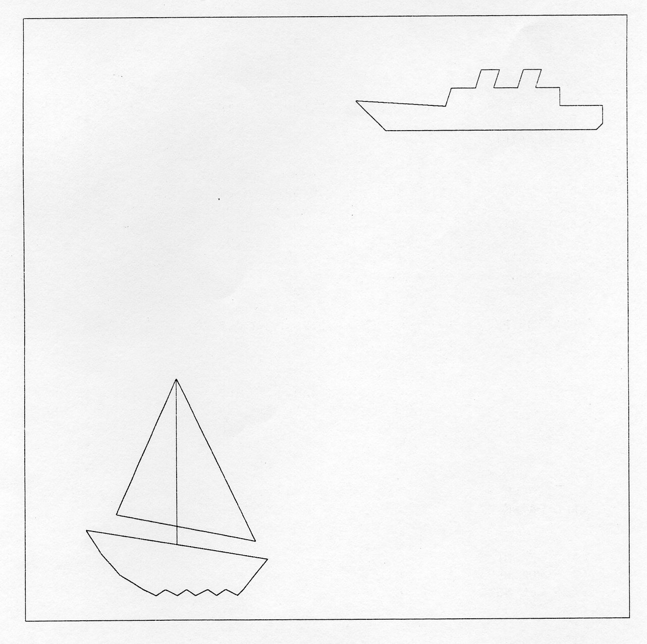
A metafile is a means of storing graphical information and reusing it in a subsequent run of GKS. Contrast this with segments which disappear when GKS is closed - except those that are sent to a metafile! Metafiles also permit the archival and export of graphics information.
The subsequent run of GKS that reads a metafile may involve a different program, a different user, a different application, a different implementation, a different language binding or even something other than GKS.
GKS provides routines for the output of data to a metafile and for the input of data from a metafile. When outputting to a metafile you address it as though it were a special form of workstation; when used in this way it is called a METAFILE OUTPUT WORKSTATION. Similarly you can input data from a metafile back into the system by accessing the metafile as though it were another workstation, and in this context it is called a METAFILE INPUT WORKSTATION.
GKS output routines will cause one or more units of data, called METAFILE ITEMS, to be written to the file. When reading a metafile, one item will be retrieved from the file at a time. The different item types are identified by item numbers. The contents and format of the GKS metafile, GKSM, are described in detail in the ISO and the BSI documents [1,2], Bibliography, Appendix J. Implementation-specific details are given in Appendix B and details of metafile workstations in Appendix C.
Output to a metafile is via a special category of workstation (MO) which is opened and closed by the same functions as other workstations. As with other workstations, output is stored while the metafile workstation is active.
Before opening the workstation, you can execute a FORTRAN OPEN statement in your program to create a sequential file and connect it to your chosen FORTRAN I/O unit. This will enable you to choose your own name for the file. See Appendix B for a discussion about the relevant OPEN statement parameters on your system.
At OPEN WORKSTATION, GKS checks to see if the connection has been made. If it has not, GKS will execute the FORTRAN OPEN. The file will then take the default system name corresponding to the given I/O unit.
A workstation type in RAL GKS for output of the GKS metafile, for instance, is 50, so a typical OPEN WORKSTATION call might be:
CALL GOPWK ( 1, 8, 50 )
Here workstation number 1 has been nominated for metafile output. At this point a metafile header record is sent to the system file that is connected to FORTRAN unit 8. Note that for metafile workstations the connection identifier is always the FORTRAN unit number.
Graphical data will automatically be sent to a metafile after the workstation has been activated. Geometric data is stored in a form equivalent to NDC. The concepts of clipping rectangle and clipping indicator are contained in one metafile item that specifies a clipping rectangle. Segment functions corresponding to GKS level 1 are simply stored on a metafile without evaluation. Since control and segment functions are stored on a metafile as they are called, the MO workstation is an audit trail of the session for output-related functions.
There is one GKS routine that is only used with category MO workstations. You can send non-GKS data to a metafile by using the special function WRITE ITEM TO GKSM (GWITM). Items produced in this way are called application data items, or USER ITEMS.
GWITM (kwkid, mftype, ncmfrd, lmfdr, mfdr)
This routine sends the data record mfdr (which is a CHARACTER*80 array of length lmfdr) to workstation kwkid. nmcfdr is the number of characters in the data record. The type of record (which will be returned when the file is scanned by GET ITEM as described in the next section) is recorded as mftype. Note that this function can only be used to transfer non-graphical information to a metafile. The item type can be any value greater than 100.
The routine is supplied to allow user data to be stored alongside its related graphics data, for the convenience of archiving and processing by the application program. It is recommended that the item should contain a key at the beginning to identify the kind of user data stored. In this way, unknown user data items can be identified if the metafile is processed by a different application program or a different system.
Example 7.1 shows a simple program that has simultaneous output to a metafile and a terminal.
      PROGRAM WRITER
*                                 GKS Example Program 7.1
      INTEGER MOUT
*                                 The FORTRAN unit number used to connect the
*                                 metafile is system-dependent; see Appendix B for
*                                 details of the values which are valid on each
*                                 system.
      PARAMETER (MOUT = fmioun)
*                                 Declare metafile output workstation values
      CHARACTER*80 MFDR(1)
*                                 Data for Ship's outline
      INTEGER NSHIP
      PARAMETER (NSHIP = 18)
      DATA XSHIP/0.20,0.10,0.40,0.42,0.50,0.52,0.58,0.56,0.64,
    :            0.66,0.72,0.70,0.78,0.78,0.92,0.92,0.90,0.207
      DATA YSHIP/0.12,0.22,0.20,0.26,0.26,0.32,0.32,0.26,0.26,
    :            0.32,0.32,0.26,0.26,0.20,0.20,0.14,0.12,0.12/
*                                OPEN GKS, OPEN and ACTIVATE WORKSTATION. The
*                                parameters for OPEN GKS and OPEN WORKSTATION
*                                are system- and device- dependent; see Appendix B
*                                for details of the values which are valid on each
*                                system.
      CALL GOPKS (kerrfl, -1)
      CALL GOPWK (1 , kconid, kwtype)
      CALL GACWK (1)
*                                End of standard opening sequence
*----------------------------------------------------------------------------------
*                                Open a file to receive the metafile
*                                The name of the file is system-dependent; see Appendix B
*                                for details of the values which are
*                                valid on each system.
      OPEN (UNIT = MOUT, FILE = metafn, STATUS = 'NEW')
*                                OPEN and ACTIVATE a metafile output workstation
*                                as workstation 2.  The parameters for
*                                OPEN WORKSTATION are system- and device-
*                                dependent; see Appendix B for details of the
*                                values which are valid on each system.
      CAL GOPWK (2, MOUT, mwktyp)
      CALL GACWK (2)
*                               Send user data
      WRITE(MFDR(1),'(A9)'} 'SHIP DATA'
      CALL GWITM (2, 150, 9, 1, MFDR)
*                               Send graphical data
      CALL GPL (NSHIP, XSHIP, YSHIP)
*                               Closedown
      CALL GDAWK (2)
      CALL GCLWK (2)
*----------------------------------------------------------------------------------
*                               Deactivate and close workstation, close GKS
      CALL GDAWK (1)
      CALL GCLWK (1)
      CALL GCLKS
      END
Input from a metafile is via a special workstation (category MI) which is opened and closed by the same functions as other workstations.
In the case of input, the metafile already exists, that is, it resides in a named system file. You will normally have to execute a FORTRAN OPEN statement in your application program, to connect the file to your chosen FORTRAN I/O unit, before opening the workstation - see appendix B.
The workstation type in RAL GKS for input of the ASCII character-encoded GKSM is 10, so a typical OPEN WORKSTATION call might be:
CALL GOPWK (2, 9, 10)
Here, workstation number 2 has been nominated for metafile input, and from this point on metafile records can be input on unit 9. In fact, the metafile header record is read in at this time, and the first item on the metafile is made the current item.
Note that the metafile input workstation cannot be activated.
Metafile input can only be accessed by three special metafile functions: GET ITEM FROM GKSM (GGTITM), READ ITEM FROM GKSM (GRDITM), and INTERPRET ITEM (GIITM).
GGTITM (kwkid, mftype, ncmfdr)
This inspects the type of the current item mftype and the length of its data record ncmfdr, and returns them to you. The data record length is the number of 80 character elements needed to contain the item.
GRDITM (kwkid, ml, lmfdr, mfdr)
Here the application program supplies a character array mfdr consisting of lmfdr elements, each of 80 characters. The current item data is input from the metafile and returned to the application program in the data record. The actual length of the data record returned is ml; normally this should correspond to ncmfdr as returned by GGTITM. If ml is less than ncmfdr, the excess parts of the item are lost; if ml = 0 , the current item will be skipped.
After the item data record has been input, the next item on the metafile is made the current item.
It is at this stage that you can deal with any user items created at output time by WRITE ITEM TO GKSM. You can reformat the item data record of a user item by using the FORTRAN internal READ statement.
GKS allows the application program access to the item data, but you are reminded that its format and content are not part of the GKS standard. The data returned by READ ITEM FROM GKSM is in a packed internal form, and you will usually pass these items back to GKS for interpretation. The routine for this purpose is INTERPRET ITEM.
GIITM (mftype, ncmfdr, lmfdr, mfdr)
Here you supply the item type mftype, and character array mfdr consisting of lmfdr elements each of 80 characters. The number of characters in the data record is returned as ncmfdr.
The effect of this call will normally be the same as if the routine that generated the metafile item was called again. Any functions that were called to control the output workstation when creating the metafile are applied to all active workstations. Attribute items will be used for interpreting subsequent primitive items on the metafile, and they will also be applied to subsequent primitive routines called directly from your program. Items containing workstation attribute settings are used to set the workstation attributes of the workstations on which the metafile contents are displayed. The normalization transformation that applies to output primitives from the metafile is the one that was in effect when the metafile was written. The primitives will not be transformed by the current normalization transformation.
No item from the metafile can be interpreted after the metafile workstation has closed.
To obtain and execute a metafile item, all three functions are called in a loop, since INTERPRET ITEM uses data provided by GET ITEM FROM GKSM (item type and item length) and READ ITEM FROM GKSM (the item itself). The metafile end item has mftype = 0. Example 7.2 shows how the routines are used together to scan a GKS metafile.
If truncation of data occurred at input, then an attempt to interpret that item will result in error 165:- 'Content of item data record is invalid for the specified item type'.
      PROGRAM READER
*                                 GKS Example Program 7.2
      INTEGER MINP
*                                 The FORTRAN unit number used to connect the
*                                 metafile is system-dependent; see Appendix B for
*                                 details of the values which are valid on each
*                                 system.
      PARAMETER (MINP = fmioun)
*                                 Declare metafile input workstation values
      INTEGER NCMFDR, MFTYPE
      CHARACTER*80 MFDR(200)
*                                OPEN GKS, OPEN and ACTIVATE WORKSTATION. The
*                                parameters for OPEN GKS and OPEN WORKSTATION
*                                are system- and device- dependent; see Appendix B
*                                for details of the values which are valid on each
*                                system.
      CALL GOPKS (kerrfl, -1)
      CALL GOPWK (1 , kconid, kwtype)
      CALL GACWK (1)
*                                End of standard opening sequence
*----------------------------------------------------------------------------------
*                                Connect the metafile to the program
*                                The name of the file is system-dependent; see
*                                Appendix B for details of the values which are
*                                valid on each system.
       OPEN (UNIT = MINP, FILE = 'metafn', STATUS = 'OLD'} '
*                                OPEN and ACTIVATE a metafile input workstation
*                                as workstation 2.  The parameters for
*                                OPEN WORKSTATION are system- and device-
*                                dependent; see Appendix B for details of the
*                                values which are valid on each system.
       CALL GOPWK (2, MINP, mwktyp)
*                                Scan through input, calling INTERPRET
*                                ITEM to drive output workstations
   10  CALL GGTITM (2, MFTYPE, NCMFDR)
   *                             Test to see if item too long
       IF (NCMFDR.GT.16000) THEN
       WRITE(*,2000) NCMFDR
2000   FORMAT(' ITEM LENGTH = ',I3,' >16000')
*                                Skip item
       CALL GRDITM (2, 0, 200, MFDR)
       ELSE
       CALL GRDITM (2, NCMFDR, 200, MFDR)
       IF (MFTYPE.GT.100) THEN
       WRITE (*,2010) MFTYPE
2010   FORMAT (' USER ITEM ',I3,' NOT INTERPRETED BY THIS EXAMPLE1)
       ELSE
      CALL GIITM (MFTYPE, NCMFDR, 200,  MFDR)
      ENDIF
      ENDIF
      IF (MFTYPE.NE.0) GO TO 10
*                              At end of run, close MI workstation
      CALL GCLWK (2)
*----------------------------------------------------------------------------------
*                               Deactivate and close workstation, close GKS
      CALL GDAWK (1)
      CALL GCLWK (1)
      CALL GCLKS
      END
GKS specifies how metafiles are to be written and read: the GKS document contains the complete definition of the interface to and from the metafile. Further, as an interim measure, the document suggests one method of storing the metafile, the GKSM. It should be noted, however, that the contents and format of the GKSM are not part of the standard.
Another metafile that can be used by RAL GKS is the Computer Graphics Metafile, CGM. This was finalised after GKS had become a standard, and, unlike the GKSM, it is a full ISO standard [6], Bibliography, Appendix J. You are recommended to use this metafile in preference to the GKSM (see Appendix C).
Nearly all the GKS output functions are recorded in the GKSM, and it is, in this sense, an 'audit trail' of the graphics session. The CGM, on the other hand, is a 'picture description' file. It describes static pictures. No functions that change pictures are included (e.g. no GKS segment functions; GKS must perform all segment functions to create the final picture which is then recorded on the CGM). These differences should not, however, be readily apparent to the user.
GKS keeps a. definition of the capability and state of the graphics system. You can inquire these values and use them to:
Some of these ideas are illustrated later in this chapter.
Some inquiries have already been touched on in earlier chapters. Many inquiries are the counterpart of some SET routine which may have been described previously. You might find it useful to look back at the previous examples and see how inquiries have been used.
There are a large number of inquiries and no attempt will be made to describe them all here. Many form groups, and the group as a whole is described. For full details, you should consult the GKS Reference Manual.
Errors detected by inquiry routines are reported by returning an error indicator. The ERROR HANDLING routine is NOT called. In the following routine descriptions the error indicator will be written as kerror.
Inquiries may be divided into three types.
Firstly there are workstation independent inquiries, such as the current fill area style index or whether a segment is open.
Secondly the are inquiries concerning the description of a particular workstation type, such as its maximum display size or how many colours it supports.
Finally there are inquiries concerning a single open workstation such as the contents of a particular fill area bundle or whether the workstation is activated.
These inquiries apply to the current state of GKS as a whole and not to any particular workstation. Much of the data obtained by these inquiries is stored in what is called the GKS State List.
Certain GKS routines can only be carried out if GKS is in a certain state. For example you can't draw any primitive unless there is a workstation that is activated.
There is a variable in the GKS state list called the GKS state value. It takes one of the following values:
where the parameters GGKCL, GGKOP, GWSOP, GWSAC and GSGOP are defined in a parameter file (see Appendix B).
The routine INQUIRE OPERATING STATE VALUE
GQOPS (jopsta)
returns this value in jopsta. In example 8.1 the state of GKS is inquired and printed.
      PROGRAM INQSTA
*                              GKS Example Program 8.1
*                              The following variable(s) are defined in the
*                              included file
*                              GGKCL, GGKOP, GWSOP, GWSAC, GSGOP
                               include GKS parameter file - see Appendix B for details
      INTEGER JOPSTA
      INTEGER     KSEGNM
      PARAMETER ( KSEGNM = 1 )
      CHARACTER *35 STATE(GGKCL:GSGOP)
      DATA STATE(GGKCL) /(GKS closed'/
      DATA STATE(GGKOP) /'GKS open'/
      DATA STATE(GWSOP) /'At least one workstation open'/
      DATA STATE(GWSAC) /'At least one workstation active'/
      DATA STATE(GSGOP) /'Segment open'/
      WRITE(*,*} 'Example 8.1'
      WRITE(*,*)
      CALL GQOPS (JOPSTA)
      WRITE{*,*) STATE(JOPSTA)
      CALL GOPKS (kerrfl, -l)
      CALL GQOPS (JOPSTA)
      WRITE(*,*) STATE(JOPSTA)
      CALL GOPWK (1, kconid, kwktyp)
      CALL GQOPS (JOPSTA)
      WRITE(*,*) STATE(JOPSTA)
      CALL GACWK (1)
      CALL GQOPS (JOPSTA)
      WRITE(*,*) STATE(JOPSTA)
      CALL GCRSG (KSEGNM)
      CALL GQOPS (JOPSTA)
      WRITE(*,*) STATE(JOPSTA)
      CALL GCLSG
      CALL GQOPS (JOPSTA)
      WRITE(*,*) STATE(JOPSTA)
      CALL GDAWK (1)
      CALL GQOPS (JOPSTA)
      WRITE(*,*) STATE(JOPSTA)
      CALL GCLWK (1)
      CALL GQOPS (JOPSTA)
      WRITE(*,*) STATE(JOPSTA)
      CALL GCLKS
      CALL GQOPS (JOPSTA)
      WRITE(*,*) STATE(JOPSTA)
      STOP
      END
The output from this program should be:
Example 8.1
GKS closed
GKS open
At least one workstation open
At least one workstation active
Segment open
At least one workstation active
At least one workstation open
GKS open
GKS closed
You may inquire about the capabilities of the GKS implementation that you are working on.
The routine INQUIRE LEVEL OF GKS:
GQLVKS (kerror, jlevel)
returns the jlevel of GKS as an integer (one of the values GLOA, GLOB, GLOC, GL1A, GLIB, GL1C, GL2A, GL2B or GL2C). For example a value of GL2B would indicate that this was a level 2b implementation. Indeed this is the level of the RAL GKS implementation. This inquiry can assist you in writing programs that will run on all GKS systems. For instance, you could detect that the system in use did not support segments (output level 0) and either not use segments or emulate them in your own program. The alternative is to attempt an operation and to let a GKS error occur if it is not available at this level. This is poor for two reasons.
The routine INQUIRE LIST ELEMENT OF AVAILABLE WORKSTATION TYPES:
GQEWK (n, kerror, navwk, kwtype)
returns an available workstation type for each value of n from one to navwk. One workstation must always be available so a value of one for n will always return a workstation type and the number of workstation types. A possible use of this inquiry would be produce a menu of output devices for selection. Example 8.2 illustrates this by printing out a list of types. The actual list of workstations types is machine-dependent (Appendix B).
      PROGRAM WKTYP
*                            GKS Example Program 8.2
      INTEGER N, KERROR, NAVWK, KWTYPE
      CALL GOPKS (kerrfl, -1)
      CALL GQEWK (1, KERROR, NAVWK, KWTYPE)
      IF (KERROR .NE. 0) THEN
       WRITE(*,*) 'Failed to Inquire First Workstation Type'
      ELSE
       WRITE(*,*) 'The following ', NAVWK,
     : ' workstation types are available1
       WRITE(*,*)
       WRITE(*,*) KWTYPE
       DO 1 N = 2, NAVWK
        CALL GQEWK (N, KERROR, NAVWK, KWTYPE)
        IF (KERROR .NE. 0) THEN
         WRITE{*,*) 'Failed to Inquire Workstation Type ', N
         GO TO 1
        ELSE
         WRITE(*,*) KWTYPE
        END IF
  1     CONTINUE
      END IF
      CALL GCLKS
      END
The output from this program could be:
THE FOLLOWING 17 WORKSTATION TYPES ARE AVAILABLE
10
50
101
102
103
104
105
106
109
110
201
203
700
701
702
703
704
The routine INQUIRE WORKSTATION MAXIMUM NUMBERS:
GQWKM (kerror, mxopwk, mxacwk, mxaswk)
returns the maximum number of open workstations mxopwk, maximum number of active workstations mxacwk and maximum number of workstations associated with a segment mxaswk. In this implementation these numbers will all be the same.
There is a limit to the number of normalisation transformations that can be stored. To avoid errors that would arise from this limit being exceeded you can INQUIRE MAXIMUM NORMALIZATION TRANSFORMATION NUMBER by calling:
GQMNTN (kerror, maxtrn)
The value maxtrn returned is the maximum normalization transformation number allowed. Thus transformations 0 to maxtrn may be used and 1 to maxtrn may be set.
There are range of inquiries, you can make about GKS as it currently is in the running of your program. These are about such things as:
The routines INQUIRE SET MEMBER OF OPEN WORKSTATIONS and INQUIRE SET MEMBER OF ACTIVE WORKSTATIONS:
GQOPWK    (n, kerror, nopwk,  kwkid)
GQACWK    (n, kerror, nacwk,  kwkid)
provide the nth workstation identifier kwkid in the list of open or active workstations, and the number of open workstations nopwk or active workstations nacwk.
Examples of inquiries on current primitive attributes are INQUIRE POLYMARKER INDEX and INQUIRE TEXT ALIGNMENT:
GQPMI        (kerror, kpmi)
GQTXAL       (kerror, jtah, jtav)
GQPMI returns kpmi, the current polymarker index, and is a natural counterpart to SET POLYMARKER INDEX (GSPMI). GQTXAL returns jtah, the horizontal text alignment. This may be GAHNOR, GALEFT, GACENT or GARITE. It also returns jtav, the vertical text alignment, which may be GAVNOR, GATQP, GACAP, GAHALF, GABASE or GABOTT. These GA.. values are defined in a parameter file (see Appendix B).
Examples of inquiries on current individual attributes are INQUIRE POLYLINE COLOUR INDEX and INQUIRE ASPECT SOURCE FLAGS:
GQPLCI      (kerror, kplcol)
GQASF       (kerror, jasf)
The polyline colour index kplcol as returned by GQPLCI will be used by GKS in line drawing if the polyline colour index ASF (aspect source flag) is set to GINDIV. You can inquire the state of this ASF by calling GQASF and checking the value of jasf (GAPLCI). In example 8.3 the main routine calls routine SHIPDW which draws the ship using individual attributes. This attempts to produce exactly the same output on any workstation. In practice a workstation may not be capable of some or all of the attribute settings; in that case a suitable action will be taken to ensure reasonable output is produced. The state of the ASFs and some individual attributes are inquired at the start of SHIPDW so that they can be reset before leaving.
      PROGRAM INDIV
*                                OPEN GKS, OPEN and ACTIVATE WORKSTATION. The
*                                parameters for OPEN GKS and OPEN WORKSTATION
*                                are system- and device- dependent; see Appendix B
*                                for details of the values which are valid on each
*                                system.
      CALL GOPKS (kerrfl, -1)
      CALL GOPWK (1 , kconid, kwtype)
      CALL GACWK (1)
*                                End of standard opening sequence
*----------------------------------------------------------------------------------
      Call SHIPWD
*----------------------------------------------------------------------------------
*                               Deactivate and close workstation, close GKS
      CALL GDAWK (1)
      CALL GCLWK (1)
      CALL GCLKS
      END

      SUBROUTINE SHIPWD
*                               Draw a ship using individual
*                               attributes.
*                               The following variable(s} are defined in the
*                               included file
*                               GINDIV, GLSOLI
*                               include GKS parameter file - see Appendix B for details
*                               Set up parameters with names for the AFSs
      INTEGER GALN, GALWSC, GAPLCI
      PARAMETER (GALN=1, GALWSC=2, GAPLCI=3)
      INTEGER JASF(13), LASF1, LASF2, LASF3, KPLCOL, LNTYPE, KERROR
      REAL WIDTH
*                               Data for Ship's Outline
      INTEGER NSHIP
      PARAMETER (NSHIP = 18)
      REAL XSHIP(NSHIP), YSHIP(NSHIP)
      DATA XSHIP/0.20,0.10,0.40,0.42,0.50,0.52,0.58,0.56,0.64,
    :            0.66,0.72,0.70,0.78,0.78,0.92,0.92,0.90,0.207
      DATA YSHIP/0.12,0.22,0.20,0.26,0.26,0.32,0.32,0.26,0.26,
    :            0.32,0.32,0.26,0.26,0.20,0.20,0.14,0.12,0.12/
*
*                               JASF   Aspect Source Flags
*                               LASF1-3 SAVED VALUES OF LASF
*                               KPLCOL   Saved Polyline Colour index
*                               LNTYPE  Saved line type
*                               KERROR Error indicator
*                               WIDTH  Saved linewidth scale factor
*                               Find current settings
      CALL GQASF (KERROR,JASF)
      IF (KERROR.GT.0) GO TO 1
      LASF1 = JASF(GALN)
      LASF2 = JASF(GALWSC)
      LASF3 = JASF(GAPLCI)
      CALL GQLN (KERROR, LNTYPE)
      IF (KERROR.GT.0) GO TO 1
      CALL GQPLCI (KERROR, KPLCOL)
      IF (KERROR.GT.0) GO TO 1
      CALL GQLWSC (KERROR, WIDTH)
      IF (KERROR.GT.0) GO TO 1
*                                Set individual attributes
      JASF(GALN)   = GINDIV
      JASF(GALWSC) = GINDIV
      JASF(GAPLCI) = GINDIV
      CALL GSASF (JASF)
      CALL GSLN  (GLSOLI)
      CALL GSPLCI (1)
      CALL GSLWSC (2.0)
*                                Draw the ship
      CALL GPL(NSHIP, XSHIP, YSHIP)
*                                Reset to original settings
      JASF(GALN)   = LASF1
      JASF(GALWSC) = LASF2
      JASF(GAPLCI) = LASF3
      CALL GSASF(JASF)
      CALL GSLN   (LNTYPE)
      CALL GSPLCI (KPLCOL)
      CALL GSLWSC (WIDTH)
  1   CONTINUE
      END

There are inquiries you can use to find out about capability and default values for a particular workstation type. All these inquiries contain the an argument kwtype, which corresponds to a particular workstation type, which must be supported by this implementation of GKS.
You can INQUIRE WORKSTATION CATEGORY and INQUIRE WORKSTATION CLASSIFICATION:
GQWKCA     (kwtype, kerror, jwkcat)
GQWKCL     (kwtype, kerror, jwkcla)
where the CATEGORY jwkcat may be:
The CLASSIFICATION jwkcla describes the type of display hardware:
The routine INQUIRE DISPLAY SPACE SIZE:
GQDSP (kwtype, kerror, jdunit, px, py, lx, ly)
returns the display surface size in device coordinate units (px, py) and in raster units (lx, ly). The device coordinates are in metres if jdunit is returned as GMETRE, and some other units if jdunit is returned as GOTHU.
INQUIRE DYNAMIC MODIFICATION OF WORKSTATION ATTRIBUTES:
GQDWKA     (kwtype, kerror, jplbun, jpmbun, jtxbun, jfabun, jparep,
            jcolrp, jwktr)
provides a list of the workstation's ability to respond graphically to a change of attributes. Each of the parameters:
may be returned as immediate (GIMM) or implicit regeneration (GIRG). If, for example, jplbun is returned as GIMM then the workstation is able to reflect any change of polyline bundle representation at once. If it is GIRG then the workstation will have to perform an implicit regeneration in order to reflect the change graphically.
You may set the deferral mode and implicit regeneration mode. They will be initialised by OPEN WORKSTATION to values which are workstation type dependent. You can obtain these default settings by INQUIRE DEFAULT DEFERRAL STATE VALUES:
GQDDS (kwtype, kerror, jdefmo, jregmo)
The deferral mode (jdefmo) may be GASAP, GBNIL, GBNIG or GASTI. The implicit regeneration mode may take the values GSUPPD or GALLOW. A pen plotter, for example, would have jregmo as suppressed because the regeneration would be slow and would waste paper.
You may find the quantity of space available to store information about the state of any particular workstation by calling INQUIRE MAXIMUM LENGTH OF WORKSTATION STATE TABLES:
GQLWK (kwtype, kerror, mplbte, mpmbte, mtxbte, mfabte, mpate, mcolte)
INQUIRE xxx FACILITIES return the capabilities of the workstation to perform a function. In this group of routines, xxx = POLYLINE, POLYMARKER, TEXT, FILL AREA, PATTERN and COLOUR. For example INQUIRE POLYLINE FACILITIES:
GQPLF (kwtype, n, kerror, nlt, lntype, nlw, widnom, widmin, widmax, nppli)
returns the nth element lntype in the list of available linetypes (as specified by n), the number of available linewidths nlw, the nominal linewidth widnom, the range of linewidths widmin to widmax and the number of predefined polyline indices nppli.
You can obtain contents of any predefined bundle by INQUIRE PREDEFINED xxx REPRESENTATION where XXX is POLYLINE, POLYMARKER, TEXT, FILL AREA, PATTERN and COLOUR. For example INQUIRE PREDEFINED COLOUR REPRESENTATION:
GQPCR (kwtype, kcol, kerror, red, green, blue)
returns the red, green blue intensities of colour kcol.
Generalized Drawing Primitive (GDP) inquiries consist of INQUIRE LIST ELEMENT OF AVAILABLE GENERALIZED DRAWING PRIMITIVES and INQUIRE GENERALIZED DRAWING PRIMITIVE.
INQUIRE LIST ELEMENT OF AVAILABLE GENERALIZED DRAWING PRIMITIVES:
GQEGDP (kwtype, n, kerror, ngdp, kgdpid)
returns the number of available GDPs ngdp and the nth GDP identifier kgdpid.
INQUIRE GENERALIZED DRAWING PRIMITIVE:
GQGDP (kwtype, kgdpid, kerror, nbundl, jbunda)
returns for GDP identifier kgdpid the number of sets of attributes used (nbundl) and a list of attributes used (jbunda(l:4)). Each of the first nbundl elements of the array jbunda will be set to one of the values GPLATT, GPMATT, GTXATT or GFAATT.
INQUIRE NUMBER OF SEGMENT PRIORITIES SUPPORTED:
GQSGP (kwtype, kerror, nsegpr)
returns the number of segment priorities in nsegpr. A value of zero means that an infinite number are available.
The ability of a workstation to reflect segment attribute changes immediately is provided by INQUIRE DYNAMIC MODIFICATION OF SEGMENT ATTRIBUTES:
GQDSGA (kwtype, kerror, jsgtr, jvonof, jvofon, jhigh, jsgpr, jadd, jsgdel)
The attributes are:
The parameters can have the same values (GIMM, GIRG) as for GQDWKA.
You can inquire the number of input devices for each class by calling INQUIRE NUMBER OF AVAILABLE LOGICAL INPUT DEVICES:
GQLI (kwtype, kerror, nlcd, nskd, nvld, nchd, npkd, nstd)
For each class of input device there is an inquiry to obtain the default data. These have names INQUIRE DEFAULT xxx DEVICE DATA. For example INQUIRE
DEFAULT LOCATOR DEVICE DATA:
GQDLC    (kwtype, klcdnn, n, minpdr, kerror, xinloc, npet,
          kpet, earea, linpdr, inpdr)
These routines are similar to GQxxS but where GQxxS returns the current state, GQDxx returns the default state. The GQxxS routines are dealt in more detail in section 8.4.4.
These inquiries concern a single workstation, rather than GKS as a whole or a particular workstation type. These inquiries contain a workstation identifier (kwkid) which must correspond to an open workstation.
The current state of a workstation is reflected in the contents of the Workstation State List.
A workstation may not be able to provide the facilities asked of it. In that case it will choose another action. For example you might set a linewidtn scale factor of 2.0 and this is not available on that workstation. The nearest value available might be 1.5 and this value will be used. Some inquiries therefore include an option (jtype) which allows you to ask for the set (GSET) or realised (GREALI) values.
The routine INQUIRE WORKSTATION CONNECTION AND TYPE:
GQWKC (kwkid, kerror, kconid, kwtype)
returns the connection identifier kconid and workstation type kwtype as given on OPEN WORKSTATION.
INQUIRE WORKSTATION STATE
GQWKS (kwkid, kerror, jstate)
returns the workstation state jstate which may be active (GACTIV) or inactive (GINACT).
By calling INQUIRE WORKSTATION DEFERRAL AND UPDATE STATES:
GQWKDU (kwkid, kerror, jdefmo, jregmo, jempty, jfname)
you may obtain:
You can obtain a list of bundle indices from the polyline, polymarker, text, fill area and pattern bundle tables, and a list of colour indices from the colour table. These routines all have the same form: INQUIRE LIST ELEMENT OF xxx INDICES, where XXX is one of POLYLINE, POLYMARKER, TEXT, FILL AREA, PATTERN or COLOUR.
GQExxI (kwkid, n, kerror, nxxi, kxxi)
(xx = PL, PM, TX, FA, PA)
where nxxi returns the number of indices, and kxxi returns the nth index in the list.
For example INQUIRE LIST ELEMENT OF COLOUR INDICES.
GQECI (kwkid, n, kerror, ncol, kcol)
where ncol returns the number of colour table entries, and kcol returns the nth element of the list of colour indices.
Corresponding to each index of each table is a representation which may also be inquired. Examples are INQUIRE POLYLINE REPRESENTATION and INQUIRE COLOUR REPRESENTATION:
GQPLR    (kwkid, kpli, jtype, kerror, lntype, width, kplcol)
GQCR     (kwkid, kcol, jtype, kerror, red, green, blue)
where the second parameter to each routine is the bundle index.
Here is example 8.3 again; this time we draw the ship in exactly the style we desire by changing the polyline representation. Inquiries are used to make SHIPDW self contained - no permanent change to the state lists is made.
      PROGRAM INQREP
*                                OPEN GKS, OPEN and ACTIVATE WORKSTATION. The
*                                parameters for OPEN GKS and OPEN WORKSTATION
*                                are system- and device- dependent; see Appendix B
*                                for details of the values which are valid on each
*                                system.
      CALL GOPKS (kerrfl, -1)
      CALL GOPWK (1 , kconid, kwtype)
      CALL GACWK (1)
*                                End of standard opening sequence
*----------------------------------------------------------------------------------
      Call SHIPWD (1)
*----------------------------------------------------------------------------------
*                               Deactivate and close workstation, close GKS
      CALL GDAWK (1)
      CALL GCLWK (1)
      CALL GCLKS
      END

      SUBROUTINE SHIPWD (KWKID)
*                               Draw a ship using a workstation independent
*                               polyline representation. This routine produces
*                               the desired effect on workstation KWKID only.
*                               Any other active workstation will draw the ship
*                               according to its current bundle tables.
*
*                               The following variable(s} are defined in the
*                               included file
*                               GREALI, GLSOLI
*                               include GKS parameter file - see Appendix B for details
      INTEGER GKWKID
      INTEGER KPLI, KPLCOL, LNTYPE, KERROR
      REAL WIDTH
*                               Data for Ship's Outline
      INTEGER NSHIP
      PARAMETER (NSHIP = 18)
      REAL XSHIP(NSHIP), YSHIP(NSHIP)
      DATA XSHIP/0.20,0.10,0.40,0.42,0.50,0.52,0.58,0.56,0.64,
    :            0.66,0.72,0.70,0.78,0.78,0.92,0.92,0.90,0.207
      DATA YSHIP/0.12,0.22,0.20,0.26,0.26,0.32,0.32,0.26,0.26,
    :            0.32,0.32,0.26,0.26,0.20,0.20,0.14,0.12,0.12/
*                             KPLI   Polyline index
*                             KPLCOL Saved Polyline Colour index
*                             LNTYPE Saved line type
*                             KERROR Error indicator
*                             WIDTH  Saved linewidth scale factor
*                             Find current settings
      CALL GQPLI(KERROR, KPLI)
      IF (KERROR.GT.0) GO TO 1
      CALL GQPLR(KWKID, KPLI, GREALI, KERROR, LNTYPE, WIDTH, KPLCOL)
      IF (KERROR.GT.0) GO TO 1
*                             Set representation
      CALL GSPLR(KWKID, KPLI, GLSOLI, 2.0, 1)
*                             Draw the ship
      CALL GPL(NSHIP, XSHIP, YSHIP)
*                             Reset to original settings
      CALL GSPLR(KWKID, KPLI, LNTYPE, WIDTH, KPLCOL)
    1 CONTINUE
      END
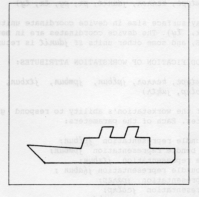
Suppose you wish to produce two strings as a single line of text. The simplest way would be to join the two strings together and produce it from a single call of GTX. This is not always possible, for example you might want to change the font, colour or some other attribute between the two strings. To do this, you can produce the first string at (x,y) and change the text attributes, but then comes the problem: Where do you put the second string?
There is a routine that tells you where to put it.
GQTXX (kwkid, x, y, text, kerror, cpx, cpy, txexpx, txexpy
The TEXT point (x,y) of the first string text and the first string itself are given to obtain the text point of the second string (cpx,cpy) (the CONCATENATION point). In addition, the coordinates of the box (txexpx,txexpy) that encloses text are given as output.
The arrays txexpx(l:4) and txexpy(l:4) are the coordinates of the corners of the TEXT EXTENT BOX, in anticlockwise order.
The output is correct if the error number kerror is zero.
The following figure shows GQTXX being used to concatenate a series of strings into a single sloping line, while attributes are changed. The text extent boxes are shown.
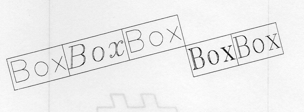
The first four strings have VERTICAL ALIGNMENT GABOTT and the remaining two have VERTICAL ALIGNMENT GATOP. This shows that the text extent box height is the top to bottom distance.
NOTE: The concatenation point is determined on the assumption that the HORIZONTAL ALIGNMENT of the next string is GAHNOR. Any other alignment would require information about the next string, if it differed in effect from normal alignment.
      PROGRAM CHNGTX
*                               The following variable(s) are defined in the
*                               included file
*                               GSTRKP
                                include GKS parameter file - see Appendix B for details
      REAL CPX, CPY, CTX, CTY, BOXX(4)/ BOXY(4)
*                                OPEN GKS, OPEN and ACTIVATE WORKSTATION. The
*                                parameters for OPEN GKS and OPEN WORKSTATION
*                                are system- and device- dependent; see Appendix B
*                                for details of the values which are valid on each
*                                system.
      CALL GOPKS (kerrfl, -1)
      CALL GOPWK (1 , kconid, kwtype)
      CALL GACWK (1)
*                                End of standard opening sequence
*----------------------------------------------------------------------------------
*                                Set text bundles
      CALL GSTXR (1,4,-104,GSTRKP,1.0,0.0,1)
      CALL GSTXR (1,5,-105,GSTRKP,1.0,0.0,1)
      CALL GSTXR (1,6,-106,GSTRKP,1.0,0.0,1)
*                                Set text index and character height
      CALL GSTXI(4)
      CALL GSCHH  (0.018)
      CALL GTX (0.1, 0.7, 'You can use routine')
*                                Inquire text extent, change text index (font)
*                                and continue from the concatenation point
      CALL GQTXX (1,0.1, 0.7, 'You can use routine', IER, : CPX,CPY , BOXX,BOXY)
      IF (IER.NE.0) GO TO 1
      CALL GSTXI (6)
      CALL GTX (CPX,CPY, ' GQTXX ')
*                                Inquire text extent, return to original text index
*                                and continue from the concatenation point
      CALL GQTXX (1,CPX,CPY,' GQTXX ', IER, CTX,CTY, BOXX,BOXY)
      IF (IER.NE.0) GO TO 1
      CALL GSTXI (4)
      CALL GTX (CTX,CTY,'to')
      CALL GTX (0.1, 0.6, 'change the ')
*                                Inquire text extent, set a new text index (font)
*                                and continue from the concatenation point
      CALL GQTXX (1,0.1, 0.6, 'change the ',IER, CPX,CPY, BOXX,BOXY)
      IF (IER.NE.0) GO TO 1
      CALL GSTXI (5)
      CALL GTX (CPX,CPY, 'font')
*                                Inquire text extent, return to original text index
*                                and continue from the concatenation point
      CALL GQTXX (1,CPX,CPY,'font',IER, CTX,CTY, BOXX,BOXY)
      IF (IER.NE.0) GO TO 1
      CALL GSTXI (4)
      CALL GTX (CTX,CTY,' or some other')
*                                new line
      CALL GTX (0.1, 0.5,'text')
*                                Inquire text extent, change character height
*                                and continue from the concatenation point
      CALL GQTXX (1,0.1, 0.5,'text',IER, CPX,CPY, BOXX,BOXY)
      CALL GSCHH (0.027)
      CALL GTX (CPX,CPY,' attribute')
*                                Inquire text extent, return to original character
*                                height and continue from the concatenation point
      CALL GQTXX (1,CPX,CPY,' attribute ',IER, CTX,CTY, BOXX,BOXY)
      CALL GSCHH (0.018)
      CALL GTX (CTX,CTY,'within a line.')
    1 CONTINUE
*----------------------------------------------------------------------------------
*                               Deactivate and close workstation, close GKS
      CALL GDAWK (1)
      CALL GCLWK (1)
      CALL GCLKS
      END
You can find the current workstation window and viewport by calling INQUIRE WORKSTATION TRANSFORMATION:
GQWKT (kwkid, kerror, jtus, rwindo, cwindo, rviewp, cviewp)
If the workstation transformation update state (jtus) is pending (GPEND), the current workstation window and viewport (cwindo (1:4), cviewp (1:4)) will not be equal to the requested values (rwindo (1:4), rviewp (1:4)). If jtus is not pending (GNPEND), the requested and current values will be equal (see Section 3.7).
CREATE SEGMENT creates a segment on all active workstations. Hence a workstation may not be storing all the segments known to GKS. The routine INQUIRE SET MEMBER OF SEGMENT NAMES ON WORKSTATION:
GQSGWK (kwkid, n, kerror, nsegnm, ksegnm)
returns the number of segment names nsegnm on workstation kwkid and the nth segment name ksegnmin the set.
INQUIRE xxx DEVICE STATE returns the state of an input device of class xxx, where xxx is one of LOCATOR, STROKE, VALUATOR, CHOICE, PICK or STRING. Examples are INQUIRE LOCATOR DEVICE STATE and INQUIRE STRING DEVICE STATE:
GQLCS     (kwkid, klcdnr, jtype, minpdr, kerror, jmode, jesw, ktnr,
           xinloc, yinloc, kpet, earea, linpdr, inpdr)
GQSTS     (kwkid, kstdnr,  minpdr, kerror, jmode, jesw, listr, istr,
            kpet, earea, mc, inipos,  linpdr, inpdr)
Some input parameters are given for all device state inquiries workstation identifier (kwkid and device number (klcdnt and kstdnr uniquely select a device. The dimension of the data record is also specified. Inquiries on LOCATOR and STROKE also have the option SET or REALISED (jtype). Inquiries on STROKE also specify the dimension (n) of the arrays used to return an initial value. Parameters that are returned by all inquiries are:
Other parameters are device class dependent. For example, LOCATOR returns the initial normalization transformation number (ktnr) and the initial locator position in world coordinates (xinloc,yinloc). More details may be found in Chapter 5.
There exist a class of inquiries concerning the display surface. All these are pixel inquiries.
INQUIRE PIXEL ARRAY DIMENSIONS
GQPXAD (kwkid, px, py, qx, qy, kerror, lx, ly)
returns the dimensions lx, ly of the pixel array implied by the two points P(px,py) and Q(qx,qy) where P is the upper left corner and Q is the lower right corner in world coordinates. Pixel rows and columns are counted if and only if they have pixel centres inside this box. The result is not effected by any segment transformation.
You can use this inquiry to make a CELL ARRAY have exactly one pixel for each cell so producing a quicker and neater image. It could also be used for drawing smooth curves with polyline on a raster device of any resolution without an excessive number of vertices.
The following two inquiry functions need only be supported by raster devices with pixel readback capability:
INQUIRE PIXEL ARRAY can be used to inquire the colour indices of all the pixels in a defined rectangular region.
GQPXA (kwkid, px, py, mx, my, isc, isr, nx, ny, kerror, jinvva, kcola)
The point (px,py) specifies (in world coordinates) the upper left corner of the region of interest; nx and ny denote the number of pixels to be interrogated across and down the display, respectively. The colour indices are returned in the mx by my array kcola. You may choose to store the colour indices in a sub-array of kcola. To do this set isc and isr to the start column and row respectively, making sure that isc and isc+nx-1 both lie between 1 and mx, similarly with isr, ny and my.
If the colour index corresponding to a particular pixel is unavailable, (for example if the point (px,py) is transformed in such a manner that pixel in question is not on the display surface), then the corresponding element of kcola. is set to -1. If any pixel data are unavailable, the flag jinvva is set to PRESENT (jinvva = GPRSNT), which denotes the presence of invalid data; otherwise it is set to ABSENT (jinvva = GABSNT). If the device is incapable of providing the required data (for example it is not an open workstation or it has no pixel readback capability), then kerror returns an error number which indicates why the data is unavailable; otherwise kerror is returned with value 0.
INQUIRE PIXEL
GQPX (kwkid, px, py, kerror, kcol)
returns the colour index of an individual pixel into kcol. The point (px,py) is specified in world coordinates.
It is equivalent to calling GQPXA with nx=ny=isc=isr=mx=my=1 and ignoring jinvva.
Within the design of any program it is important to consider what action to take if an exceptional condition (exception) occurs. An exception might be due to illegal data or an error in the code which calls GKS.
Most GKS routines have a number of error conditions. Some of these are defined by the GKS ISO standard, some by the FORTRAN 77 language binding, while the remainder are implementation dependent. For a full list of error messages see Appendix A.
If a problem is detected by an inquiry routine, it returns an error indicator containing a GKS error number. All other GKS routines report errors by calling the GKS Error Handler
GERHND (kerrno, kfi, kerfil)
which, by default, calls the GKS Error Logger
GERLOG (kerrno, kfi, kerfil)
For both of these routines, kerrno is the function identifier, kfi is the function identifier and kerfil is the error file. The function identifier is a machine dependent integer.
The routine GERLOG produces an error message of the form:
NAME [NUMBER] ERROR MESSAGE
where NAME is the name of the GKS routine you called, NUMBER is the GKS error number and ERROR MESSAGE is a description of the problem. For example, an attempt to run example program DIRCOL (which is intended for a colour device) on a monochrome terminal would result in the report
GSPC [ 86] Colour index is invalid
If GKS is open the report will appear on the error stream, as specified on OPEN GKS (GOPKS). Otherwise the report will be output on the default output stream.
After detecting an exception, GKS might decide that it is unable to continue. The GKS function EMERGENCY CLOSE GKS (routine GECLKS) would be called and an attempt made to complete any graphics produced so far. If you decide to abandon your program, you might also wish to call GECLKS. The actions performed are
All GKS routines, apart from the inquiries, report errors by calling the GKS Error Handler (routine GERHND). By default this routine calls the GKS Error Logger (routine GERLOG) which produces the error report. GKS allows you to replace the error handler, but not the error logger. Your own version of the error handler may or may not call the error logger as you wish. Your error handler must follow some simple rules.
A typical use of your own error handler is shown in example 9.1. A copy of the error number is placed in common MYCOM and the Error Logger then called. The non-GKS routine that follows (MYERR) returns the error status and clears it to zero. If MYERR is called after each GKS routine the argument will always contain the last error reported.
      SUBROUTINE GERHND{IERNO, IDENT, IERFIL)
      INTEGER IERNO, IDENT, IERFIL
      INTEGER MERNO
      COMMON /MYCOM/ MERNO
*                                Save error number
      MERNO = IERNO
*                                Report error
      CALL GERLOG(IERNO, IDENT, IERFIL)
      END
      SUBROUTINE MYERR(IERNO)
      INTEGER IERNO
      INTEGER MERNO
      COMMON /MYCOM/ MERNO
*                                Return error number
      IERNO = MERNO
*                                Reset error status
      MERNO = 0
      END
ACCUMULATE TRANSFORMATION MATRIX [6.4.1] ACTIVATE WORKSTATION [4.2] ASSOCIATE SEGMENT WITH WORKSTATION [6.11.2] ASF [8.2.3] Aspect Source Flags [2.3.3] [8.1.3] Attributes [2.2] - Segment [6.4] BUNDLED [2.9] Bundled Attributes [2.2.1] CELL ARRAY [2.1] [2.7] CHAR precision text [2.5.3] Character expansion factor [2.5.5] [2.5.6] [2.5.8] Character height [5.6] Character spacing [4.2] [6.5] CHOICE [5.6] CLEAR WORKSTATION [4.2] [6.5] Clipping [3.5] CLOSE GKS [4.1] CLOSE SEGMENT [6.3] CLOSE WORKSTATION [4.2] CGM [7.4] Colour [2.2.3] [2.10] - Index [2.2.3] - Table [2.2.3] Computer Graphics Metafile [7.4] Connection identifier [4.2] Coordinate Systems [3.1] - Switch [6.4.1] Coordinates, Normalized Device [3.3] Coordinates, World [3.2] COPY SEGMENT TO WORKSTATION [6.11.2] CREATE SEGMENT [6.3] Cursor Pattern [5.9.3] DEACTIVATE WORKSTATION [4.2] Deferral mode [6.9] DELETE SEGMENT [6.5] DELETE SEGMENT FROM WORKSTATION [6.5] Device Coordinates [3.7] Display Surface [3.3] - Size [5.9.1] Drawing [2.1] Echo [5.9.3] Echo area [5.9.1] Echo Switch [5.9.2] EMERGENCY CLOSE GKS [9.1.1] Error Handler [9.1] - Replacing [9.1.2] Error Logger [9.1] Errors [9] ESCAPE [4.5] EVALUATE TRANSFORMATION MATRIX [6.4.1] FILL AREA [2.1] [2.6] Fonts [2.5.3] GACTM [6.4.1] GACWK [4.2] GASGWK [6.11.1] GCA [2.7] GCLKS [4.1] GCLRWK [4.2] GCLSG [6.3] GCLWK [4.2] GCRSG [6.3] GCSGWK [6.11.2] GDAWK [4.2] GDSG [6.5] GDSGWK [6.5] GECLKS [9.1.1] GENERALIZED DRAWING PRIMITIVE (GDP) [2.1.2] Geometric attributes [2.5] [2.6.2] GERHND [9.1] GERLOG [9.1] GESC [4.5] GET ITEM FROM GKSM [7.3] GEVTM [6.4.1] GFA [2.6.1] GGSLCM [5.9.2] GGDP [2.8.1] GGTITM [7.3] GIITM [7.3] GINLC [5.9.4] GINSG [6.11.3] GKSM [7] GMSG [4.4] GOPKS [4.1] GOPWK [4.2] GPL [2.3.1] GPM [2.4.1] GPREC [4.6] GQxxF [8.3.1] GQxxR [8.3.1] [8.4] GQxxS [8.4.4] GQACWK [8.2.3] GQASF [8.2.3] GQCR [8.4] GQDXX [8.3.3] GQDDS [8.3] GQDLC [8.3.3] GQDSGA [8.3.2] GQDWKA [8.3] GQExxI [8.4] GQECI [8.4] GQEGDP [8.3.1] GQEWK [8.2.2] GQGDP [8.3.1] GQLCS [8.4.4] GQLI [8.3.3] GQLVKS [8.2.2] GQLWK [8.3] GQMNTN [8.2.2] GQOPS [8.2.1] GQOPWK [8.2.3] GQPCR [8.3.1] GQPLCI [8.2.3] GQPLF [8.3.1] GQPLR [8.4] GQPMI [8.2.3] GQPX [8.4.5] GQPXA [8.4.5] GQPXAD [8.4.5] GQSGP [8.3.2] GQSGWK [8.4.3] GQSTS [8.4.4] GQTXAL [8.2.3] GQTXX [8.4.1] GQWKC [8.2.3] GQWKCA [8.3] GQWKCL [8.3] GQWKDU [8.4] GQWKM [8.2.2] GQWKS [8.4] GQWKT [8.4.2] GRDITM [7.3] GRENSG [6.6] GRQCH [5.6] GRQLC [5.3] GRQSK [5.4] GRQST [5.8] GRQVL [5.5] GRSGWK [6.10.2] GSASF [2.9] GSCHH [2.5.7] GSCHSP [2.5.7] GSCHUP [2.5.9] GSCHXP [2.5.8] GSCLIP [3.5] GSCR [2.10] GSDS [6.9] GSDTEC [6.7.2] GSELNT [3.2] GSFACI [2.6.5] GSFAI [2.6.3] GSFAIS [2.6.5] GSFAR [2.6.3] GSFASI [2.6.5] GSHLIT [6.4.3] GSLN [2.3.3] GSLWSC [2.3.3] GSMK [2.4.3] GSMKSC [2.4.3] GSPA [2.6.4] GSPAR [2.6.4] GSPARF [2.6.4] GSPKID [6.7.1] GSPLCI [2,3.3] GSPLI [2.3.2] GSPLR [2.3.2] GSPMCI [2.4.3] GSPMI [2.4.2] GSPMR [2.4.2] GSSGP [6.4.4] GSSGT [6.4.1] GSTRKP [2.5.3] GSTRP [2.5.3] GSTXAL [2.5.11] GSTXCI [2.5.4] GSTXFP [2.5.3] GSTXI [2.5.5] GSTXP [2.5.10] GSTXR [2.5.5] GSVIS [6.4.2] GSVP [3.3] GSVPIP [5.3] GSWKVP [3.7] GSWKWN [3.7] GSWN [3.2] GTX [2.5.1] GUREC [4.6] GUWK [6.10.1] GWITM [7.2] HATCH, fill area [2.5.3] Highlighting, segment attribute [6.4.3] HOLLOW, fill area [2.6.3] Implicit regeneration [2.11] [6.9] [8.3] [8.4] INDIVIDUAL [2.9] Individual Attributes [2.2.2] INITIALISE LOCATOR [5.9.4] Input, Metafile [7.3] Input device - Initial values [5.9.4] - Initialisation [5.9] - Logical [5.1] - Numbers [5.2] INQUIRE - Current Individual attributes [8.2.3] - Current Primitive attributes [8.2.3] - DEFAULT XXX DEVICE DATA [8.3.3] - DEFAULT DEFERRAL STATE VALUES [8.3] - DISPLAY SPACE SIZE [8.3] - DYNAMIC MODIFICATION OF SEGMENT ATTRIBUTES [8.3.2] - DYNAMIC MODIFICATION OF WORKSTATION ATTRIBUTES[8.3] - GENERALIZED DRAWING PRIMITIVE [8.3.1] - LEVEL OF GKS [8.2.2] - LIST ELEMENT OF XXX INDICES [8.4] - LIST ELEMENT OF AVAILABLE WORKSTATION TYPES [8.2.2] - LIST ELEMENT OF AVALABLE GENERALIZED - DRAWING PRIMITIVES [8.3.1] - MAXIMUM LENGTH OF WORKSTATION STATE TABLES [8.3 ] - MAXIMUM NORMALIZATION TRANSFORMATION NUMBER [8.2.2] - NUMBER OF AVAILABLE LOGICAL INPUT DEVICES [8.3.3] - NUMBER OF SEGMENT PRIORITIES SUPPORTED [8.3.2] - OPERATING STATE VALUE [8.2.1] - PIXEL [8.4.5] - PIXEL ARRAY [8.4.5] - PIXEL ARRAY DIMENSIONS [8.4.5] - PREDEFINED xxx REPRESENTATION [8.3.1] - SET MEMBER OF ACTIVE WORKSTATIONS [8.2.3] - SET MEMBER OF OPEN WORKSTATIONS [8.2.3] - SET MEMBER OF SEGMENT NAMES ON WORKSTATION [8.4.3] - TEXT EXTENT [8.4.1] - WORKSTATION CONNECTION AND TYPE [8.4] - WORKSTATION CATEGORY [8.3] - WORKSTATION CLASSIFICATION [8.3] - WORKSTATION DEFERRAL AND UPDATE STATES [8.4] - WORKSTATION MAXIMUM NUMBERS [8.2.2] - WORKSTATION STATE [8.4] - WORKSTATION TRANSFORMATION [8.4.2] - XXX DEVICE [8.4.4] - XXX FACILITIES [8.3.1] - xxx REPRESENTATION [8.3.1] [8.4] INSERT SEGMENT [6.11.3] Interior Style [2.6.3] INTERPRET ITEM [7.3] Interpretation, Metafile [7.3] Linetype [2.3.3] Linewidth [2.3.3] - Scale factor [2.3.3] LOCATOR [5.3] Marker - Size [2.4.3] MARKER SIZE SCALE FACTOR [2.4.2] Marker Type [2.4.3] MESSAGE [4.4] Metafile - Input [7.3] - Interpretation [7.3] - Output [7.2] - Overview [7.1] - MI [7.3] - MO [7.2] Multiple Normalization Transformation [3.6] NDC [3.3] Normalisation Transformation, Selecting [3.2] Normalisation Transformation, Multiple [3.6] Normalized Device Coordinates [3.3] OPEN GKS [4.1] NDC [3.3] Normalization Transformation, Selecting [3.2] Normalization Transformations, Multiple [3.6] Normalized Device Coordinates [3.3] OPEN GKS [4.1] Open segment [6.2] OPEN WORKSTATION [4.2] Operating state [4.3] Output, Metafile [7.2] Output Primitives [2.1] PACK [4.6] PATTERN, fill area [2.6.3] [2.6.4] PICK [5.7] [6.7] Pick Identifier [6.7.1] Picture regeneration [6.10] POLYLINE [2.1] [2.3.1] Polyline Bundled Attributes [2.2.1] [2.3.2] Polyline Individual Attributes [2.2.2] [2.3.3] POLYMARKER [2.1] [2.4.1] Precision of Text [2.5.3] Priority, segment attribute [6.4.4] Prompt [5.9.3] READ ITEM FROM GKSM [7.3] REALISED value, option in inquiries [8.4 ] REDRAW ALL SEGMENTS ON WORKSTATION [6.10.2] Regeneration [6.10] RENAME SEGMENT [6.6] REQUEST CHOICE [5.6] REQUEST LOCATOR [5.3] REQUEST PICK [5.7] [6.7] REQUEST STRING [5.8] REQUEST STROKE [5.4] REQUEST VALUATOR [5.5] Segments [6.1] - Attributes [6.4] - Closing [6.3] - Creating [6.3] - Deleting [6.5] - Detectability [6.7.2] - Highlighting [6.4.3] - Priority [6.4.4] - Renaming [6.6] - Transformations [6.4.1] - Visibility [6.4.2] - Visible effects [6.8] SELECT NORMALIZATION TRANSFORMATION [3.2] SET values, option in inquiries [8.4] SET xxx MODE [5.9.1] SET ASPECT SOURCE FLAGS [2.2.2] [2.5.6] [2.6.5] [2.9] SET CHARACTER EXPANSION FACTOR [2.5.7] SET CHARACTER HEIGHT [2.5.7] SET CHARACTER SPACING [2.5.7] SET CHARACTER UP VECTOR [2.5.9] SET CLIPPING INDICATOR [3.5] SET COLOUR REPRESENTATION [2.10] SET DEFERRAL STATE [6.9] SET FILL AREA COLOUR INDEX [2.6.5] SET FILL AREA INDEX [2.6.3] SET FILL AREA INTERIOR STYLE [2.6.5] SET FILL AREA REPRESENTATION [2.6.3] SET FILL AREA STYLE INDEX [2.6.5] SET HIGHLIGHTING [6.4.3] SET LINETYPE [2.3.3] SET LINEWIDTH SCALE FACTOR [2.3.3] SET MARKER SIZE SCALE FACTOR [2.4.3] SET MARKERTYPE [2.4.3] SET PATTERN SIZE [2.6.4] SET PATTERN REFERENCE POINT [2.6.4] SET PATTERN REPRESENTATION [2.6.4] SET PICK IDENTIFIER [6.7.1] SET POLYLINE COLOUR INDEX [2.3.3] SET POLYLINE INDEX [2.3.2] SET POLYLINE REPRESENTATION [2.3.2] SET POLYMARKER COLOUR INDEX [2.4.3] SET POLYMARKER INDEX [2.4.2] SET POLYMARKER REPRESENTATION [2.4.2] SET SEGMENT DETECTABILITY [6.7.2] SET SEGMENT PRIORITY [6.4.4] SET SEGMENT TRANSFORMATION [6.4.1] SET TEXT ALIGNMENT [2.5.11] SET TEXT COLOUR INDEX [2.5.4] SET TEXT FONT AND PRECISION [2.5.3] SET TEXT INDEX [2.5.5] SET TEXT PATH [2.5.10] SET TEXT REPRESENTATION [2.5.5] SET VIEWPORT [3.3] SET VIEWPORT INPUT PRIORITY [5.3] SET VISIBILITY [6.4.2] SET WINDOW [3.2] SET WORKSTATION VIEWPORT [3.7] SET WORKSTATION WINDOW [3.7] Sloping Text [2.5.9] [2.5.10] SOLID, fill area [2.6.3] STRING, input [5.8] STRING, precision text [2.5.3] STROKE, input [5.4] STROKE, precision text [2.5.3] TEXT [2.1] [2.5.1] Text Alignment [2.5.11] Text Attributes [2.5.2] Text Colour Index [2.5.4] [2.5.5] [2.5.6] Text Font and Precision [2.5.3] [2.5.5] [2.5.6] Transformation - Matrix [6.4.1] - Segment [6.4.1] Transformation, Normalization [3.2] Transformation, Workstation [3.7] UNPACK [4.6] UPDATE WORKSTATION [6.10.1] User data [7.2] VALUATOR [5.5] Viewport [3.3] Visibility, segment attribute [6.4.2] WC [3.1] Window [3.2] WISS [6.11] WRITE ITEM TO GKSM [7.2] Workstation [4.2] - Activating [4.2] - Clearing [4.2] - Closing [4.2] - Deactivating [4.2] - Identifier [4.2] - Opening [4.2] - Type [4.2] Workstation Independent Segment Storage [6.11] Workstation Transformation [3.7] Workstation Viewport [3.7] Workstation Window [3.7] World Coordinates [3.2]
