The aim of this report is to indicate the range and quality of the work carried out on the Cray X-MP and Cray Y-MP supercomputers at the Rutherford Appleton Laboratory over the period 1991 to 1993. The material was obtained in response to a letter sent to over 160 users in May 1993 requesting contributions by October 1993.
Although the response from the different user communities was variable, we hope that the contributions give some indication of the scope of the current on the Cray vector supercomputers. We are grateful to all who contributed to this report and look forward to future reports which will highlight the growing diversity of the field.
Professor C R A Catlow
Chairman, Atlas Cray Users' Committee
January 1994
Computational methods can now make detailed and accurate predictions of the structures and properties of inorganic materials. Electronic-structure calculations are being performed on increasingly large systems, and simulation methods, based on "effective interatomic potentials", may now be used to model complex materials. One of the most exciting fields for the application of computer modelling is mineralogy. Mineralogy poses major challenges to the predictive capacity of contemporary computational techniques. But, as a discipline, mineralogy can also benefit immeasurable from the capability of computer methods (a) to simulate the inaccessible atomistic or microscopic processes that underlie macroscopic phenomena, and (b) to simulate pressure and temperature conditions normally beyond the range of experiment. Hence as a subject computational mineral physics has grown rapidly in recent years, attracting solid state physicists and chemists interested in testing and establishing their theories and methodologies on real, structurally-complex materials, and minerologists, petrologists and geophysicists who require data (currently unavailable by direct experiment) to constrain models for and to obtain insights into the processes that determine and underpin planetary evolution. Brief reference to the many papers now appearing in Earth Science journals shows how the subject as a whole is benefitting from this synergism. Below, we outline some of the topics which have been studied in the past few years, using the super computer facilities at RAL.
DEECTS AND DIFFUSION IN PEROVSKITES: We are carrying out a series of calculations on petrovskite materials, with the aim of understanding the rheology of the lower mantle. We are using the defects code CASCADE to predict the energies of defect formation and migration in perovskites. So far we have excellent quantitative agreement with known data for titanates. Recently, we have also used our atomistic computer simulation techniques to investigate the site partitioning of iron in (MgFe)SiO, petrovskites. Our calculations predict that the most energetically favourable reaction for iron substitution will be a direct exchange of Fe2+ for Mg2+. Substitution of Fe into the octahedral site and Si into the 8-12 fold coordinated site, as recently proposed by Jackson and co-workers, is predicted to be extremely unlikely. This conclusion has just been confirmed by MAS NMR (Kirkpatrick et al., (1991) Amer Mineral, 76, p 673).
DEFECT FORMATION VOLUMES IN MgO: The variation of the activation volume and free energy of formation of Schottky defects in MgO have been investigated with PARAPOCS. The approach used is based on the construction of a charge neutral supercell of atoms containing the defect, which is equilibrated ( within the limits of the quasi-harmonic approximation) at the required P and T. The results demonstrate that the supercell method works well. We predict that both the activation volume and free energy formation of Schottky defects in MgO are highly dependent on pressure, but only weakly affected by temperature. The activation volume is predicted to decrease by more than 50% as the pressure increases to that in the lower mantle. Moreover, the assumption used by many previous workers that the activation volume has the same pressure dependence as the atomic volume has been shown to be incorrect. We have recently extended this work to include the calculation of diffusion coefficients in MgO using Vineyard theory.
MOLECULAR DYNAMIC & THERMODYNAMIC MODELS OF MELTING: Work has begun to extend the phenomenological dislocation model of melting, successfully used by Poirier to model Fe, to other metallic systems. The model assumes that a melt is isostructural with the crystal saturated with dislocation cores. By considering the volumetric dilation introduced by dislocations in a metal, estimates of the entropy and volume of melting can be obtained. So far excellent agreement has been obtained for over 12 metals between the observed melting temperature and that predicted by our model. This finding underpins the validity of Poirier's work on the melting of Fe and its geophysical implications. We propose to extend our study to consider the melting of silicates.
Molecular dynamics offers the only approach to understanding melting at an atomic level. We are using both constant T and constant P molecular dynamics to investigate the details of melting and pre-melting processes in MgO and MgSiO3-perovskite. Our calculations (based on empirical potentials) predict reasonable volumes of melting, but the absolute temperature of melting seems to be overestimated by 500 to 1000K. We are particularly interested in investigating the effects of defects and surfaces on the predicted melting behaviour of materials, as these will destabilize the crystal and hence encourage melting at lower temperatures than predicted for the perfect bulk. We are also studying the effect of pressure on the structures of the melts produced in these systems. We have again confirmed the pre-melting enhanced oxygen mobility in the perovskite lattice, and will carry out further investigations into the nature of superionic conduction in perovskites. Work on fluoride perovskites is also in hand to widen the basis of our analysis of the pre-melting behaviour of perovskite-structure phases.
THE LIMITS OF THE QUASI-HARMONIC APPROXIMATION: Our code PARAPOCS performs free energy minimization using interatomic potentials, and so enables the thermodynamic properties of a silicate to be calculated from their predicted lattice dynamical characteristics. The approach depends upon the validity of the quasiharmonic approximation, which is known only to hold at temperatures below the Debye temperature of the crystal. Above this temperature, phonon-phonon interactions become significant, and in the past quantitative simulations in this regime have required the use of molecular dynamics (MD) techniques. MD, however, cannot usually be used with the more sophisticated potentials used in lattice dynamical calculations. We are carrying out a series of parallel calculations using both methods to establish firmly the point at which the quasi-harmonic approximation collapses for mantle materials. We are particularly interested in the effect of pressure on this, since it is known that pressure suppresses intrinsic anharmonic processes, and so at depth in the mantle, the quasi-harmonic approximation may become valid over a wide temperature range. Our preliminary conclusions, from calculations at simulated geothermal temperatures, are that for geophysical systems the quasi-harmonic approximation will only become valid at pressures greater than 100 GPa.
THE EFFECT OF P ON THERMAL EXPANSION: Recent experimental work has shown that the pressure dependence of the thermal expansion coefficient can be expressed as (α/α0) = (V0/V)-δT , where δT, the Anderson-Gruneisen parameter, is approximately independent of pressure, and for the materials studied has a value that lies between 4 and 6. Calculation of δT from seismic data, however, appears to suggest a contradictory value of between 2 and 3 for mantle-forming phases. Using an atomistic model based on our previously successful many-body interatomic potential set (THB1), we have performed calculations to obtain values of δT for four major mantle-forming minerals. Our model results are in excellent agreement with experimental data, yielding values of between 4 and 6 for forsterite and MgO, and values in the same range for MgSi03-perovskite and Mg2SiO44-spinel. The apparent conflict between the values of δT predicted from seismic data and those obtained from experiment, and now from theory, must be due to invalid approximations in the complex inversion of the seismic data.
THE VIBRATIONAL SPECTRA AND THERMODYNAMICS OF MINERALS: We have used the PARAPOCS code to model the vibrational properties of crystal lattices, which are subsequently used to interpret infra-red and Raman data obtained on perovskites, MgSiO3 and Mg2SiO4 polymorphs, etc. The use of such microscopic models is the only way to fully assign the spectra of such complex structures. We have also used this free energy code to predict the phase diagram for a number of ABO3 systems, and to calculate oxygen isotope equilibria. We have just started to use this lattice dynamical code to establish the microscopic basis for many of the approximations used in the variety of definitions of the Gruneisen parameter.
Al/Si DISORDER AND THE MULLITE PROBLEM: Modelling disorder is much more difficult than modelling an ordered system, and modelling an incommensurate phase is much more difficult than modelling a normal material. Hence simulating mullite, which involves both disorder and an incommensurate structure represents a major challenge. We have now established a methodology for modelling disorder, and are now approaching the problem of simulating what are considered to be the key defects in the mullite structure (namely the so-called T-T-T* cluster). We propose to pursue this work and extend it to modelling Al/Si disorder in other silicates, and particularly in feldspars.
AB INITIO CALCULATIONS ON MINERALS: Modelling of atomic interactions requires an accurate description of interatomic forces. It is now possible to perform quantum mechanical calculations on complex phases, from which insights into bonding, and hence accurate interatomic potential models, can be derived. We are investigating the suitability of the code CRYSTAL (C Pisani et al, Lecture Notes in Chemistry, vol 48, Springer-Verlag) as a way of performing such quantum mechanical calculations. CRYSTAL enables calculations (with periodic boundary conditions) to be carried out, within the limits of the Hartree-Fock approximation. In addition, in association with Dr Renata Wentzcovitch, we have been carrying out a series of quantum mechanical molecular dynamics calculations to predict the structure and stability of MgSiO3 polymorphs as a function of pressure.
G D Price, I G Wood and D Akporiaye
The prediction of zeolite structures
In: Modelling of structure and reactivity in zeolites (eds C R A Catlow) Academic Press,
London (1992) 19
S Padlewski, V Heine and G D Price
Atomic ordering around oxygen vacancies in sillimanite: A model for the mullite structure
Phys Chem Minerals 18 (1992) 373
M Matsui and G D Price
Computer simulation of the MgSiO3 polymorphs
Phys Chem Minerals 18 (1992) 365
B Reynard, G D Price and P Gillet
Thermodynamic and anharmonic properties of forsterite: computer simulations vs high
pressure and high temperature measurements
J Geophys Res 97 (1992) 19791
S Padlewski , V Heine and G D Price
The energetics of interaction between oxygen vacancies in sillimanite: A model for origin of
the incommensurate structure of mullite
Phys Chem Minerals 19 (1992) 196
A Pavese, M Catti, G D Price and R A Jackson
Interatomic potentials for CaCO3 polymorphs (calcite and aragonite) fitted to elastic and
vibrational data
Phys Chem Minerals 19 (1992) 80
P Chandley, R J H Clark, R J Angel and G D Price
An investigation of the site preference of Vanadium doped into ZrSiO4 and ZrGeO4
Dalton Proceedings of the Royal Chem Soc (1992) 1579
R A Jackson and G D Price
A transferable interatomic potential for calcium carbonate
Molecular Simulation 9 (1992) 175
S Padlewski, V Heine and G D Price
A microscopic model for a very stable incommensurate modulated structure: mullite
J Phys Con Matter 5 (1993) 3417
M Catti, A Pavese and G D Price
Thermodynamic properties of CaCO3 calcite and aragonite: a quasi-harmonic calculation
Phys Chem Minerals 19 (1993) 472
R Nada, J Stuart, G D Price, C R A Catlow and R Dovesi
Comparative study of all-electron and core pseudo-potential basis sets for periodic ab initio
Hartree-Fock calculations: the case of MgSiO3-ilmenite
J Phys Chem Solids 54 (1993) 281
R M Wentzcovitch, J L Martins and G D Price
Ab initio molecular dynamics with variable cell shape: application to MgSiO3
Phys Rev Letts 70 (1993) 3947
P Gillet, F Guyot, G D Price, B Tounerie, and A LeCleach
Phase changes and thermodynamic properties of CaTiO33 Spectroscopic data,
vibrational modelling and some insights on the properties of MgSiO3 perovskite
Phys Chem Minerals 20 (1993) 159
G D Price
Computer modelling of defects and diffusion in minerals
Terra Abstracts 4 (1992) 37
L Vocadlo and G D Price
Computer calculations for absolute ionic diffusion in MgO using the supercell method
Terr Abstracts 4 (1992) 45
J H Davies and G D Price
Are the lateral thermal variations constant with depth through the interior of the
mantle
EOS 73 (1992) 61
G D Price
Molecular dynamic simulation of melting
Terra Abstracts 5 (1993) 522
An understanding of the interaction between magnetic fields and velocities in a conducting fluid is essential to our understanding of the dynamics of the Earth's core. Kinematic dynamo calculations are one important step in obtaining such an understanding; they assume that the fluid velocity is known, and solve the electromagnetic induction equation for the magnetic field produced. The numerical problem reduces to that of finding eigenvalues and eigenvectors of a large, sparse, real but non-symmetric matrix. Thus we can get some idea of the sort of fluid motions that must be occurring in the Earth to produce the observed magnetic field.
Codes we have developed solve the induction equation in a spherical shell geometry, using a truncated spherical harmonic expansion, and either a finite difference radial grid representation or a parallel shooting method. We solve both the full 3-dimensional equations, and a simplified 2-d set obtained in the nearly-symmetric limit.
Our investigations to date have involved simple, large-scale velocity fields. Even so the computational requirements of the work are fairly heavy; the low truncation limits enforced by the machine memory size and speed effectively limit the spatial resolution obtainable. Access to the Atlas Crays, and in particular the Y-MP service, has allowed us to investigate systems previously beyond our resolution, resulting in worthwhile new findings which will be published in the near future. (One paper submitted to Nature, another in preparation for the Journal of Fluid Mechanics).
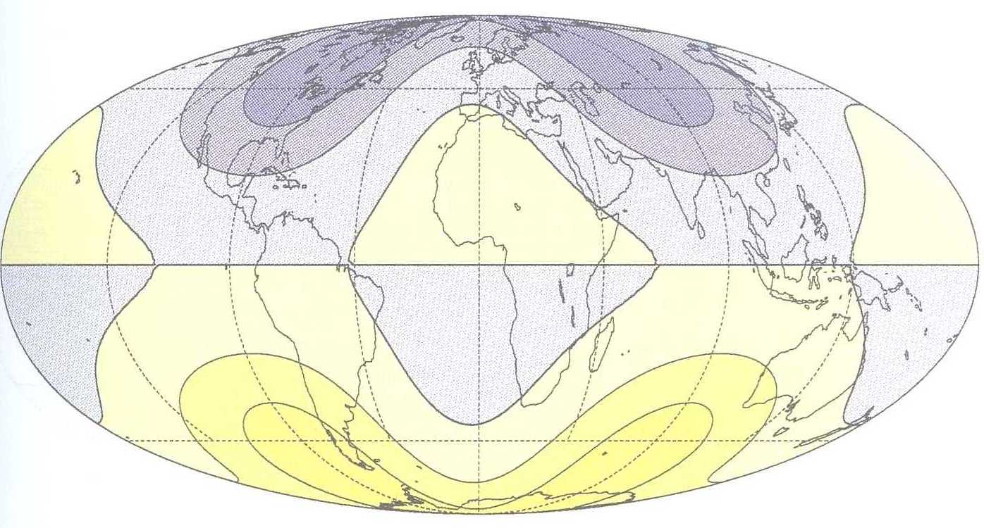
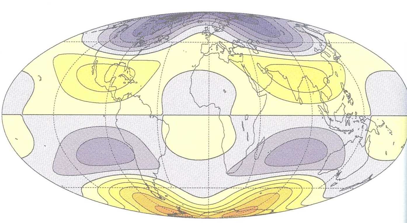
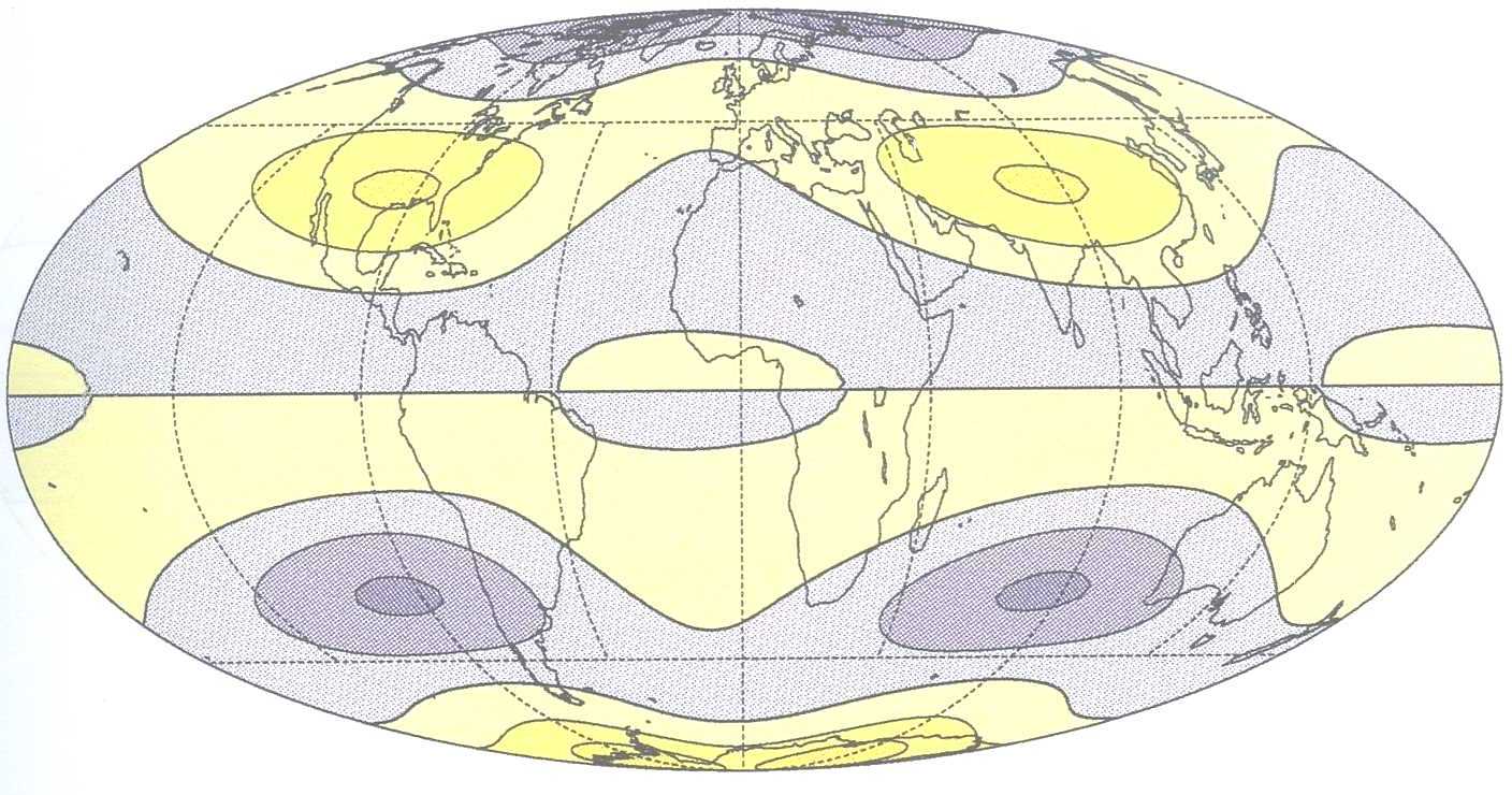
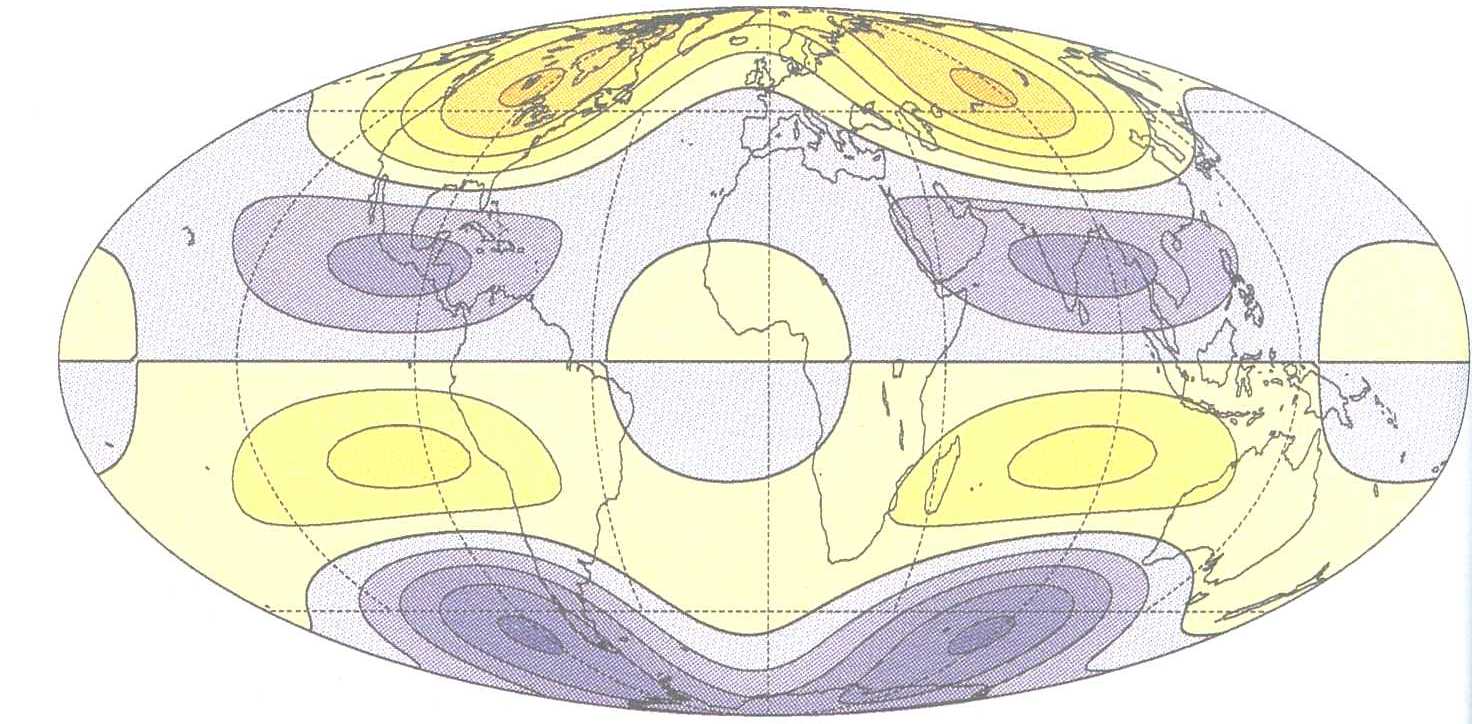
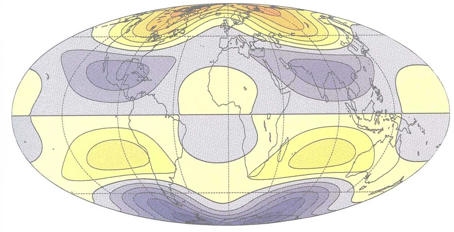
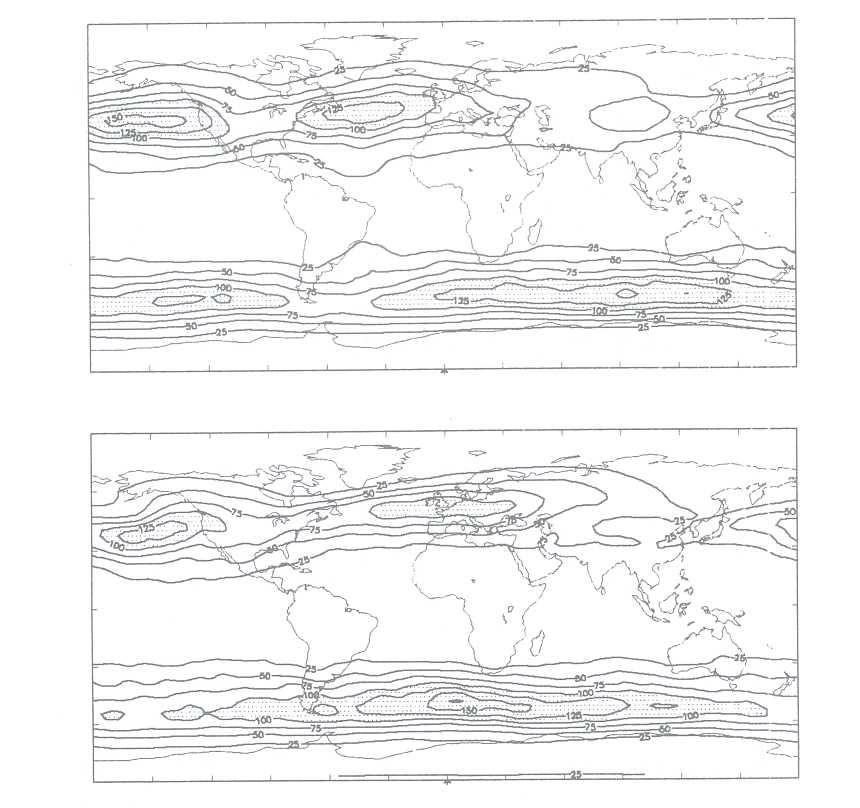
Recent work has focused on the role of meridian circulation in determining the time-dependence of the magnetic field: the presence of such an overturning circulation tends to stabilise an oscillatory magnetic field. The point at which the change-over in stability from stationary to oscillatory solutions occurs has been investigated in some detail, and we hope that it will shed new light on the reversal behaviour of the Earth's magnetic field. The figures enclosed show examples of the radial magnetic field at the outer surface of the dynamo region, for both stationary and oscillatory fields, from work carried out on the Y-MP Cray.
It is hoped that future work, using more realistic velocity fields, and incorporating dynamic effects, will lead to greater understanding of the interaction of planetary scale velocities and magnetic fields. Such work will require even more intensive calculations to be carried out.
The May 23, 1989 Macquarie Ridge earthquake (Mw = 8.2) was the largest to have occurred globally in the last fourteen years. In addition, it was the largest to have occurred on the plate boundary between the India/ Australia tectonic plate and the Pacific plate, south of New Zealand in more than seventy years. It is also the largest known submarine strike slip earthquake. (An earthquake is called "strike slip" if the net slip is practically in the direction of the fault strike.) At the time of the event, the newly installed worldwide distribution of seismometers were in operation. These instruments are "broad-band", that is, they have a flat response over a very broad frequency range (100s: period to 1 hz. frequency) and have a very large dynamic range, faithfully recording ground motions for magnitude 8 earthquakes at distances as close as 30°. This was therefore the largest well-recorded strike slip earthquake and offered a unique opportunity for its study in detail.
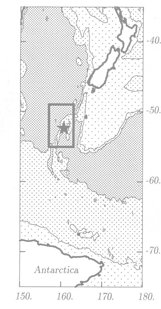
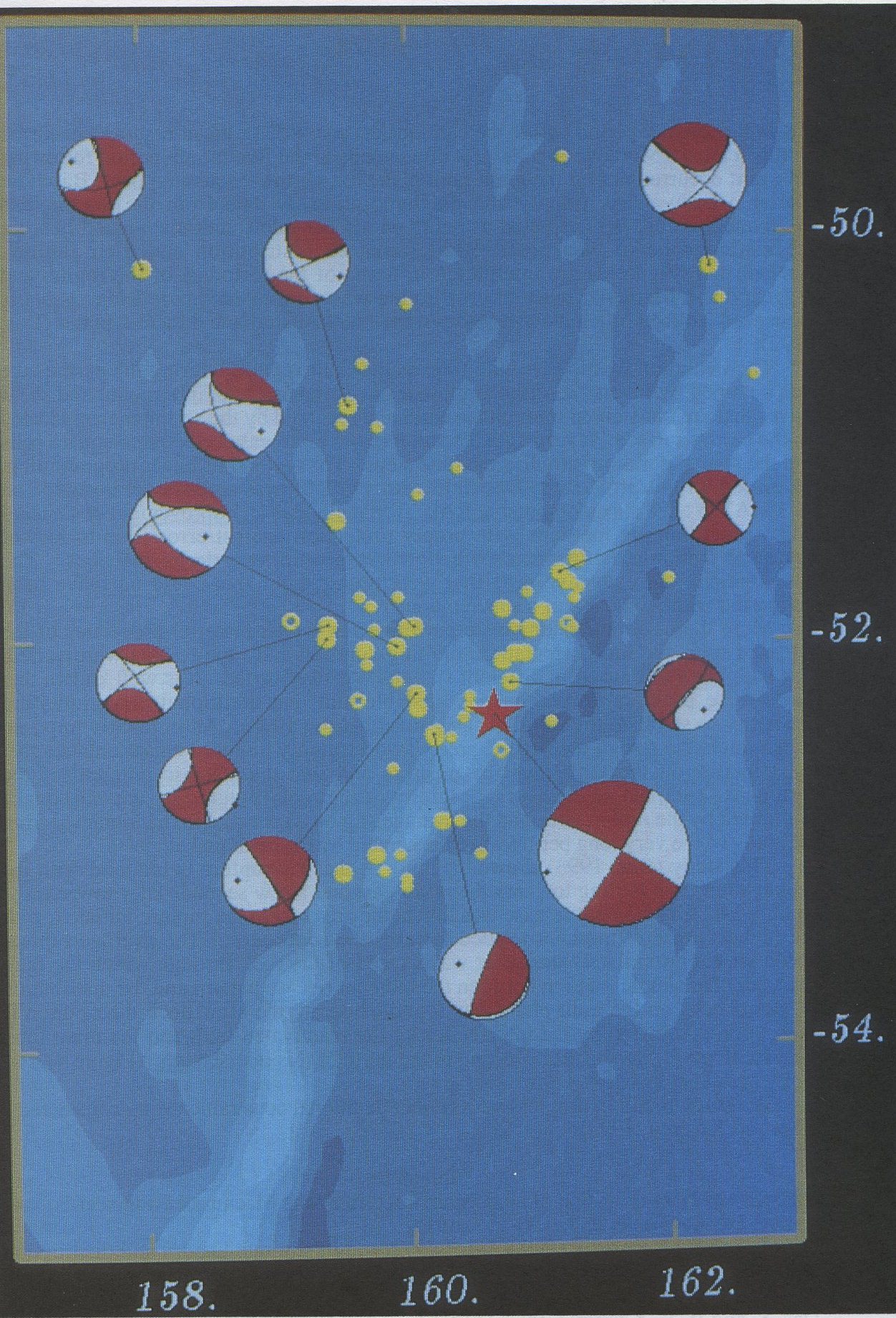
Figure 1 shows a map of the Macquarie Ridge (MR) area with bathymetric contours and the location of the Macquarie Ridge earthquake. The Macquarie Ridge is seen to extend south from South Island, New Zealand. The India/ Australian plate is subducting beneath the Pacific plate in the northern and southern parts of the MR but on the portion of the plate boundary where the 1989 event occurred the motion is primarily of strike-slip type.
The smaller events which accompany great earthquakes ("aftershocks") generally give an indication of the ruptured area of the fault. Such an aftershock study was made and shows (Figure 2) that there were remarkably few and small aftershocks for an event of this size. The aftershocks were distributed along a 220 km portion of the India/ Australia-Pacific plate boundary and indicate that the motion was bilateral on a vertical fault. In addition, the earthquake reactivated a 175 km section of a fault to its west which had been dormant at least since 1964 (as seen from the study of the seismicity on the central portion of the MR in the 25 year period before the earthquake) and 44% of the aftershocks occurred on this feature. Moreover, the largest aftershocks in the five month period following the event occurred not on the main fault plane but on the reactivated one. Based on available bathymetry, gravity and magnetic anomaly data from the region, this reactivated feature is interpreted as being an old oceanic fracture zone and hence a pre-existing zone of weakness. The aftershock distribution and their faulting mechanisms (Figure 2) are interpreted in terms of the tectonics of the region and suggest that a triangular piece of crust to the west of the Macquarie Ridge is being "squeezed" to the north and west between the India/Australia and Pacific plates (Das, 1992).
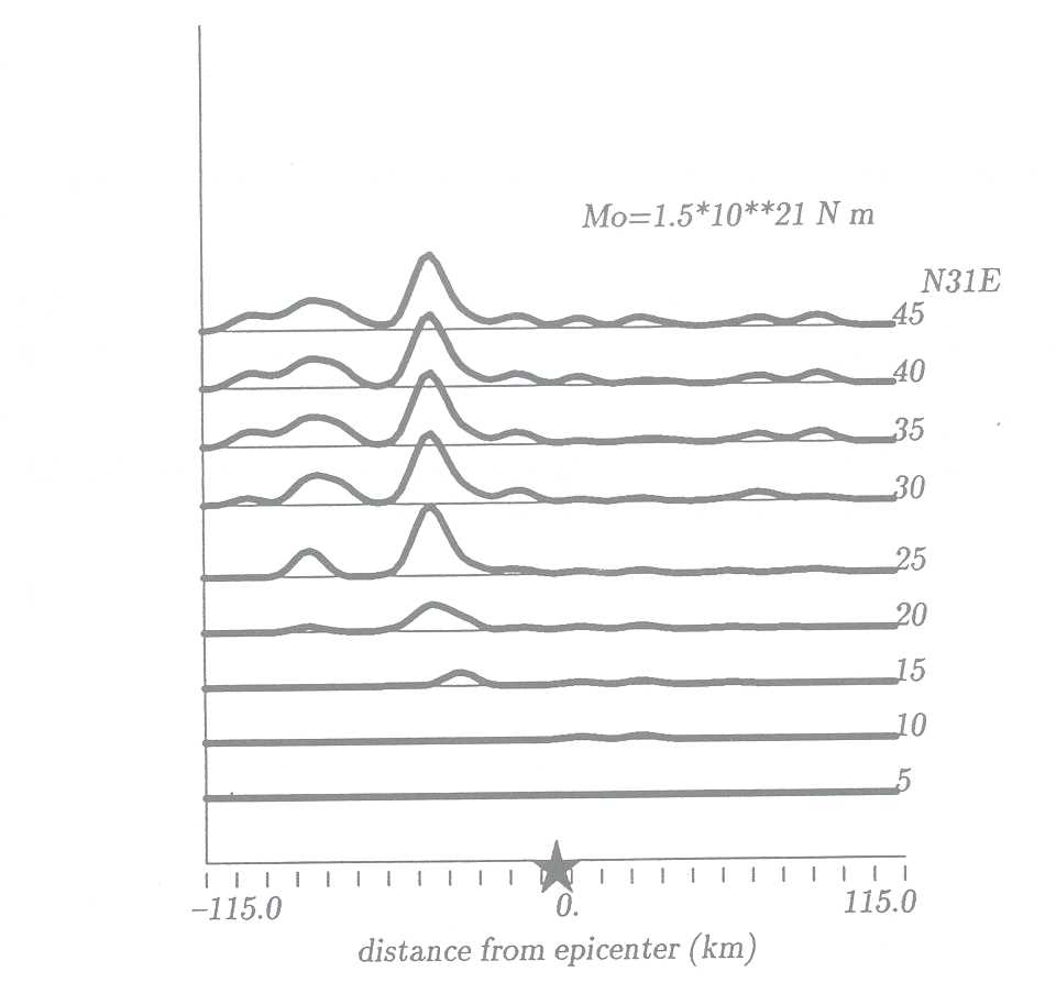
The evolution of slip rate with time as the fault ruptured during the earthquake was obtained by inversion of the amplitudes and shapes of compressional and shear waves that are transmitted through the earth and recorded by the seismometers located on the earth's surface. A rectangular section of the fault was divided into square cells and the source duration into discrete time steps. The method of linear programming, developed for this problem by Das and Kostrov (1990), was used for the inversion on the CRAY-YMP8 supercomputer at RAL. The method is an improvement of standard linear programming methods with proper protection against errors due to loss of accuracy that invariably occurs when working with very large matrices. The development and extensive tests that were required for this could not have been performed without the use of a supercomputer.
More than 100 inversions were performed in which material properties of the ruptured rock, the fault orientation, faulting duration and rupture area were varied. The weighting of data from different stations was also varied. It is well known that the inverse problem solved here is unstable and that additional constraints are necessary to stabilize the solution (Das and Kostrov, 1990). An implicitly imposed constraint is the size of the rupture area. Two explicitly imposed constraints are that the slip rate on the fault must be positive and that the seismic moment of the earthquake (defined as the average rigidity of the rock ruptured by the earthquake multiplied by the rupture area and the average slip on it) is equal to that obtained from the study of the very long period waves generated by the earthquake.
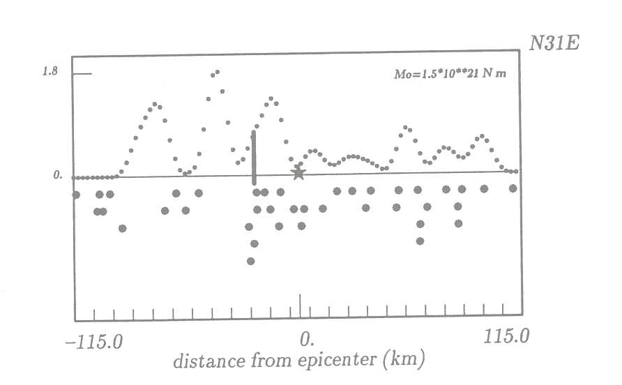
This study (Das, 1993) showed (Figure 3) that the rupture is bilateral with the propagation first starting towards the north-east and a few seconds later towards the south-west. The moment release was low in the area where the rupture initiated, with the highest areas of moment located towards the south-west. The average rupture speed was approximately the shear wave speed of the rock through which the fault ruptured. No simple relation between the moment release pattern and the distribution of aftershocks on the fault plane was found. Instead, the aftershock distribution is seen to be dominated by the intersection of the reactivated fault and the main fault plane with most aftershocks occurring to the north of this intersection. (Figure 4).
The study is still in progress with further additional constraints being considered (Das and Kostrov, 1993).
Das, S. (1992) Reactivation of an oceanic fracture by the Macquarie Ridge earthquake of 1989, Nature, 357, 150-153, 1992.
Das, S. and B.V. Kostrov (1990) Inversion for fault slip rate history and distribution using linear programming. The 1986 Andreanof Islands earthquake, J. Geophys. Res., 95, 689 9-6913, 1990.
Das, S. and B. V. Kostrov (1993) Diversity of solutions of the problem of earthquake faulting inversion. Application to SH waves from the great 1989 Macquarie Ridge earthquake, Phys. Earth Planet Int., preprint.
Das, S. (1993) The Macquarie Ridge earthquake of 1989, Geophys. J. Int., in press.
Das, S. Reactivation of an oceanic fracture by the Macquarie Ridge earthquake of 1989 Nature 357 (1992) 150-153.
Das, S. The Macquarie Ridge earthquake of 1989, Geophys. J. Intl. (1993) in press.
Das, S. and B. V. Kostrov Diversity of solutions of the problem of earthquake faulting inversion. Application to SH waves from the great 1989 Macquarie Ridge earthquake ( 1993) preprint.
The UK Universities Global Atmospheric Modelling Programme (UGAMP) is a community research project funded by NERC. UGAMP is a collaboration between six universities; Cambridge, East Anglia, Edinburgh, London (Imperial College), Oxford and Reading as well as the Rutherford Appleton Laboratory.
UGAMP's aim is to improve our basic understanding of a variety of large scale atmospheric phenomena and processes that are important in predictions of our climatic-chemical environment, thereby advancing the ability to simulate them correctly in models of the climate system. UGAMP's approach is to use controlled experiments with a hierarchy of models of varying degrees of complexity as research tools to further basic understanding.
The UGAMP science plan is ambitious and broad and it concerns the wealth of important atmospheric problems that need to be solved. It therefore covers a wide range of research areas, one of which is paleoclimate modelling. Predictions for climate change have been developed in the context of our current climate. However predictions are required for parameters outside this range and one very demanding test of such models is to apply them to past climates. The last glacial cycle (up to 120kyr before present) should prove an especially good test for the models because there is relatively good data coverage. This is particularly true for the last glacial maximum for which there is extensive land and sea coverage.
It is now widely accepted that the primary driving force of our Quaternary glacial/interglacial climate cycles is the change of seasonal distribution of insolation induced by orbital parameter changes. These changes are periodic, occurring at approximately 20, 40 and 100 kyr periods. However the climatic response to these forcings is currently a maximum at the 100kyr period, whereas the dominant forcing is at the 20 and 40 kyr periods. Thus feedback processes must be important and the strongest of these is thought to be related to the growth of the ice sheets.
Of central importance to the growth of ice sheets is the mass balance, which strongly depends on the simulated temperature and precipitation patterns. These are a function of elevation and the general circulation. In particular, the mid-latitude depressions (especially the storm tracks) play a vital role in transporting heat, moisture and momentum towards the pole and onto the ice sheets.
In order to accurately model mid-latitude depressions, general circulation models (GCM) have to be used. These types of models cannot be run for 100,000 years. Instead a "snapshot" of the typical climate of a particular period is obtained, having given it the appropriate boundary conditions. These include the ice sheet extent and elevation, the orbital parameters, the atmospheric CO2 concentration, and for an atmospheric GCM, the sea surface temperature. The model is then run for up to 10 simulated years and the results can be diagnosed. In the following section, we will describe preliminary results for a simulation of the last glacial maximum, 21 kyr BP.
The GCM that is used for this study is based on the UGAMP General Circulation Model (UGCM). The UGCM has been adapted for long-range climate simulations starting from the high resolution weather forecasting model developed and used by the European Centre for Medium-range Weather forecasts
The model is modified to include the ice sheet and sea surface temperature reconstructions of CLIMAP (1981). The model is spectral and the spectral coefficients are truncated at total wavenumber 42 (corresponding to a horizontal grid of 128 × 64 longitudes/latitudes). This is the first time that such a high resolution model has been used for simulations of the last glacial maximum. The model also includes a seasonal cycle. Previous results from perpetual February and August simulations were reported in Valdes and Hall(1993).
Figure 1 shows the model simulation of mean surface air temperature (at a height of 2m above surface) for the December - February season for (a) present day and (b) LGM conditions. The 0°C isotherm approximately shows the limit of the sea ice and is prescribed from the CLIMAP data set. The present day surface temperatures are remarkably good. This is particularly true for the Arctic region. Observations of January surface temperatures (Schutz and Gates, 1971), show Arctic regions dropping to -25 to -35°C, very similar to the model simulations. Similarly, land temperatures over the US and Eurasia are close to observations. Southern hemisphere temperatures are not quite so realistic. The model has Antarctic temperatures dropping as low as -50°C, whereas observations suggest temperatures nearer -35°C. However, this discrepancy occurs only in areas of high orography. In regions of low elevation, the model is closer to observations.
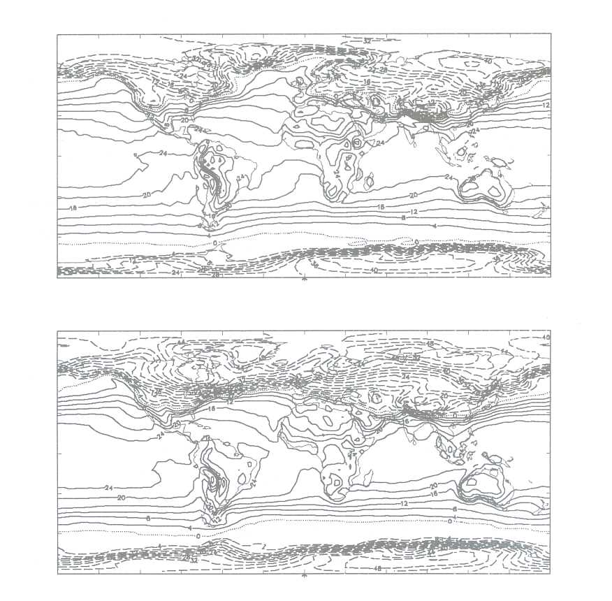
The simulation for the LGM shows enhanced temperature gradients in the Northern hemisphere, particularly over the Northern Atlantic. In these regions, the temperatures have dropped by up to 40°C. This is comparable to previous studies (e.g. Joussaume, 1992). Temperatures decrease rapidly with distance poleward of the ice edge and the enhanced temperature gradient extends across the entire ocean. The gradient is also strong over North America. This appears, in part, to be a product of the high elevations of the Laurentide ice sheet which cools to below -56°C. Similar low temperatures are found over the Greenland and Scandinavian ice sheets.
These changes are important for the mid-latitude depressions. The altered temperature gradients in the Northern Hemisphere result in modified activity in the storm track regions. Figure 2 shows the transient eddy kinetic energy per unit mass at approximately 250 mb for (a) present day and (b) LGM conditions. This has been temporally filtered to include only the relatively fast moving mid-latitude depressions with time scales for growth and decay of the order of six days or less using the filter described in Hoskins et al., 1989.
The maxima over the Pacific, Atlantic, and Southern hemisphere oceans are commonly used as locators of the 'storm tracks'. The present day simulation is in reasonable agreement with observations (Hoskins et al., 1989). The peaks in the Pacific and Atlantic are similar to observations, but both storm tracks are further south than observed, by about 5°.
For the LGM simulation, the region of maximum eddy kinetic energy is considerably more confined meridionally, but extends much further into Europe. Thus over the Atlantic, the eddy kinetic energy is considerably reduced, whereas over Europe there is a substantial increase. This increase extends well into the continent, to 90°E. These changes are generally consistent with the changed surface temperature gradient. The temperature gradients at the edge of the sea ice result in mid-latitude depressions closely following the edge of the ice. The sharpness of the storm track is a result of the relative efficiency with which the depressions can transport heat, and the relatively narrow meridional band over which heat needs to be transferred with such strong temperature gradients.
Finally we show the total precipitation for the December-February season for (a) the present day and (b) the LGM. In mid-latitudes and especially in the European region, there is a dramatic change in the pattern. The precipitation is in a much more narrow band but, like the storm track itself, it extends considerably further into Europe. The band of precipitation closely follows the edge of the ice.
For both ice sheets, there is accumulation virtually everywhere, both in the interiors of the glaciers and at the ice edges. However, the largest changes occur at the ice edge. There is substantial accumulation over the northern Rockies, over the Eastern seaboard of the U.S.A. and over Southern Europe. This accumulation is closely related to the changes in storm tracks and precipitation already discussed. There is also net accumulation of snow over the Tibetan plateau and the edge of the Antarctic continent (not shown). The former result is of interest in that the existence of a Tibetan ice sheet is controversial (Kuhle, 1987).
This has been a very brief description of one area of research within UGAMP. This work was carried out by P.J. Valdes, N.M.J. Hall and D. Buwen at the University of Reading. It shows that a GCM can be used to understand better the atmospheric transport of moisture onto the ice sheets. The GCM used was run on the SERC YMP/8. The 10 year LGM simulation described here required approximately 450 hours of CPU time on the YMP/8 generating some 15Gbytes of data that needed to be analysed subsequently.
CLIMAP, 1981, Seasonal reconstructions of the earth's surface at the Last Glacial Maximum, Geological Soc. America, Map Chart Ser., MC-36, Boulder, Colorado.
Hoskins, BJ., H.H. Hsu, I.N. James, M. Masutani, P.D. Sardeshmukh and G.H. White, 1989: Diagnostics of the global atmospheric circulation. WRCP report 27.
Joussaume, S., 1991: Paleoclimatic tracers: An investigation using an atmospheric general circulation model under ice age conditions. Part 1: Desert dust. J. Geophys. Res. In press.
Kuhle, M., 1987: Subtropical mountain and highland glaciation as ice age triggers and the waning of the glacial periods in the Pleistocene. GeoJournal 14, p393-421.
Valdes, P.J., and Hall, N.M.J., 1993, Mid-Latitude Depressions during the last ice-age. Submitted to Proceedings of Nato Advanced Summer School on Palaeoclimates.
Severe convective storms in the Pennines, a hilly terrain in the Northwest of England, are presently under investigation by means of rain gauge and radar data and a numerical cloud physics and dynamics model. Analysis of observational data so far suggests that the orientation of the Pennines encourages destabilisation of the atmosphere through long sun-facing slopes and other structured terrain. The direction of the steering level winds in relation to the underlying topography, as well as to the surface flow, appeared to be of major importance for the development and especially the intensification of the storms. The application of a three-dimensional cloud physics model to the particular region of the Pennines is performed at present to gain more insight into the particular role of the Pennines on the outbreak and development of severe convective storms. Initial model results suggest that the juxtaposition of airmasses with different moisture contents east and west of the Pennines could be important for the intensification of thunderstorms. It is shown that the wind direction up to the steering level winds in about 700 hPa in relation to the underlying topography has major influence on the favoured locations of cell initiation. Similarly, development of urban heat island effects in the Bradford and Manchester area also have a strong impact on the outbreak of convection.
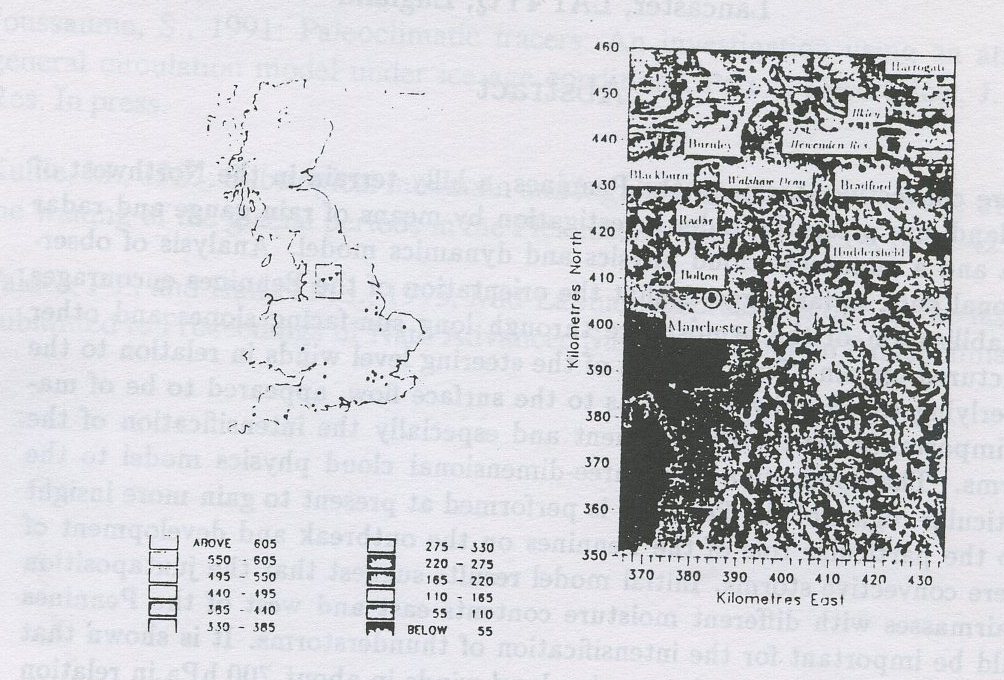
The outbreak of severe convective storms with rainfall intensities of more than 100 mm/2hrs in Britain is often considered concentrated in the lowlands of the Southeast of England; only a few have been reported in the hilly terrains of Wales, Northwest England or Scotland (Reynolds 1978). Of these few, three in Northwest England occurred in a radius of 30 km in a particular part of the hilly Central Pennines, and they rank among the 10 highest short-period rainfalls in all Britain (Fig. 1 ).
Although reports of severe convectives storms are biased towards areas of dense gauge network, the scarcity of severe storms in hilly terrain on one hand, and the spatial concentration of the few extreme rainfall events in the Central Pennines on the other hand, appears significant. The underlying study therefore aims to investigate the particular role of the Central Pennines on the initiation and further development of convective storms. At the present stage emphasis is put on the locations of cell outbreaks rather than rainfall intensities.
Analyses of the influence of the Pennines on the development of convection has been studied by means of gauge and conventional C-band weather radar data. However, the quality and resolution of both the gauge and radar data was too poor to study the subject in sufficient detail. It was therefore decided to apply a numerical model to the area. Because of the highly three-dimensional character of thunderstorms a three-dimensional model had to be chosen.
In the next section the model used for the underlying investigation is briefly described. In section 4 the set-up of the model and results of three different simulations are presented, as well as a comparison with observational data. In section 5 the results are summarised and concluded.
The model used for the underlying study was developed by T.L. Clark and improved and modified since amongst others by Clark (1977, 1979), Clark and Farley (1984), Smolarkiewicz and Clark (1986) and Clark and Hall (1991). The model has been chosen for this work because it has proved to simulate convection successfully over structured terrain over the past years.
The model is a three-dimensional second order finite difference storm model that is based on the equations of motion .
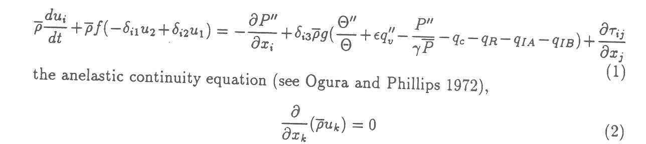
the first law of thermodynamics.
(The variables have been split into three components, the base state, x, which represent the atmospheric conditions for an idealized atmosphere of constant stability S, the difference between the constant stability atmosphere and a hydrostatically-balanced atmosphere, x'(z), and perturbations that evolve with time x"(x, t), and that actually drive the motion.)
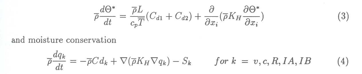
where ui are the components of wind velocity, f is Coriolis parameter, ρ is density, P is pressure, Θ is potential temperature, and x, y and z are cartesian coordinates. δij is the Kronecker symbol, g is gravitational constant, ℇ = Rv/Rd - 1 is the ratio of the gas constants for moist (Rv) and dry air (Rd) minus 1, γ = cp/cv is the ratio of the specific heat constants, qv,c,R,IA,IB are the mixing ratios of vapour, cloud water, rain water, and the two ice types A and B. KH is the eddy mixing coefficient for heat, and Cdk are evaporation, sublimation or nucleation rates, depending on the described process, and Sk is the transfer of cloudwater to rainwater. υij is the stress tensor defined as
![]()
where Km is the eddy coefficient for momentum and Dij the deformation tensor.
The surface sensible heat flux, Ss, is specified dependent upon the incident solar radiation at z=0 as
where μ(x, y) is a factor which determines the conversion rate from incoming solar radiation to sensible heat flux, So is the solar constant (1395 Wm-2), Z is the angle of the zenith angle of the sun, φ latitude, δ declination angle, H hour angle and hx,y are the gradients of topography in the east and west direction respectively. In this study, a latent heat flux, Si, has been added to the code in a similar way than the sensible heat flux, in order to account for continuous inflow of moisture. The conversion factor μ(x, y) ranged between 30 % (μ=0.3) in urban areas to account for the heat island effect, and very small (μ ≈ 0.0) above sea.
A simple method of cloud cover feedback to surface heating has also been added to the code. It was assumed that the shadow of clouds reduced the conversion of incoming solar radiation to sensible heat or latent heat by about 30% at the surface. The area shadowed by the clouds has been determined by simple geometry including the zenith angle and the azimuth angle of the sun and the dimensions and location of the cloud.
The model equations are written in terrain following coordinates following Gal-Chen and Somerville (1975), which simplify the lower vertical boundary conditions over structured terrain. The cloud and ice parameterisation of the model are based on the Koenig-Murray ice parameterisation (1976). The model has the option to nest several domains with different grid size resolutions. The information from the outer domains are used for initialisation of the inner domains at the beginning of each time step. After completion of each time step the more detailed information gained by the inner domains are fed back into the outer domains. This saves computing time and allows simulations of bigger areas.
The model has been chosen for this work because it has proved able to simulate convection successfully over structured terrain over the past years.
In the present study the newest version of the model available in June 1993 (G2TC36) has been applied. The model code contains about 36000 lines of FORTRAN code and was written for parallel processing on CRAY supercomputers, and is presently run on the YMP at the Rutherford Appleton Laboratories near Oxford. The model output is mainly graphical and uses NCAR-graphics, which has also been installed on the YMP. A simulation of 5 hours real time consumes about 5000 sec user CPU-time, and 180 sec system CPU-time.
The model simulations were aimed to investigate the role of the Pennines on the outbreak and development of convection under influence of different wind directions and surface conditions. The internal fine scale structure of individual cells was not investigated, because there was no observational data to compare and verify the numerical results with, and it would have considerably increased the computing time.
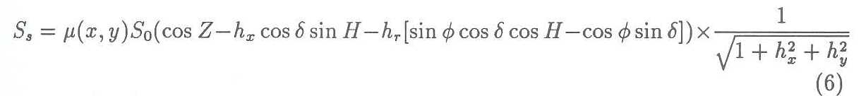
The model has been set up for this study with three nested domains. The first and outer domain extends from 215 km East and 321 km North to 599 km East and 561 km North in 12×12 km2 grid steps (Positions in National Grid Reference). At the southwest corner of the domain steep topography gradients are present due to the Welsh mountains. Test runs showed that the model copes with the elevated terrain at the boundaries, and that the topography data does not have to be smoothed in this particular area.
The second domain extends from 347 km East and 345 km North to 451 km East and 497 km North in 4×4 km2 grid steps. The second domain is not much larger than the third domain in east-west direction, because there are no major topographical features present that have to be resolved on a finer scale. In north-south direction it extends further than the innermost grid to resolve the influence of the Lake District and Yorkshire Dales, as well as of the structured terrain to the south.
The third domain extends from 359 km East and 381 km North to 435 km East and 457 km North in 2×2 km2 grid steps. Although a grid size of 2×2 km2 is still too coarse to resolve fine scale dynamic structures of convective cells, it represents a reasonable compromise between the resolution of convection and the consumption of computing time.
The topography for most parts of the two inner domains was provided by the Meteorological Office, the data for the outer domain was extracted from Ordnance Survey maps.
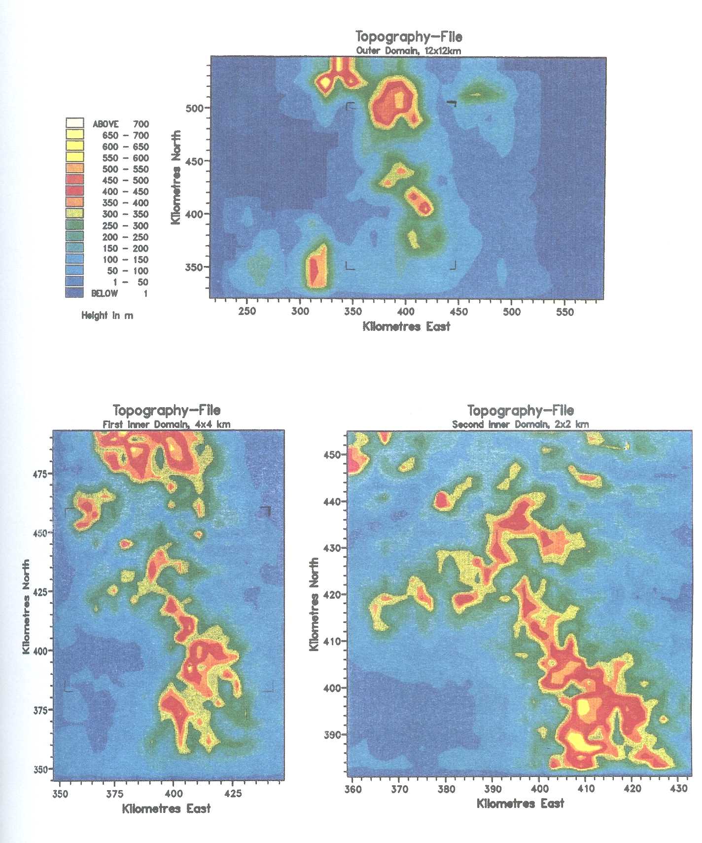
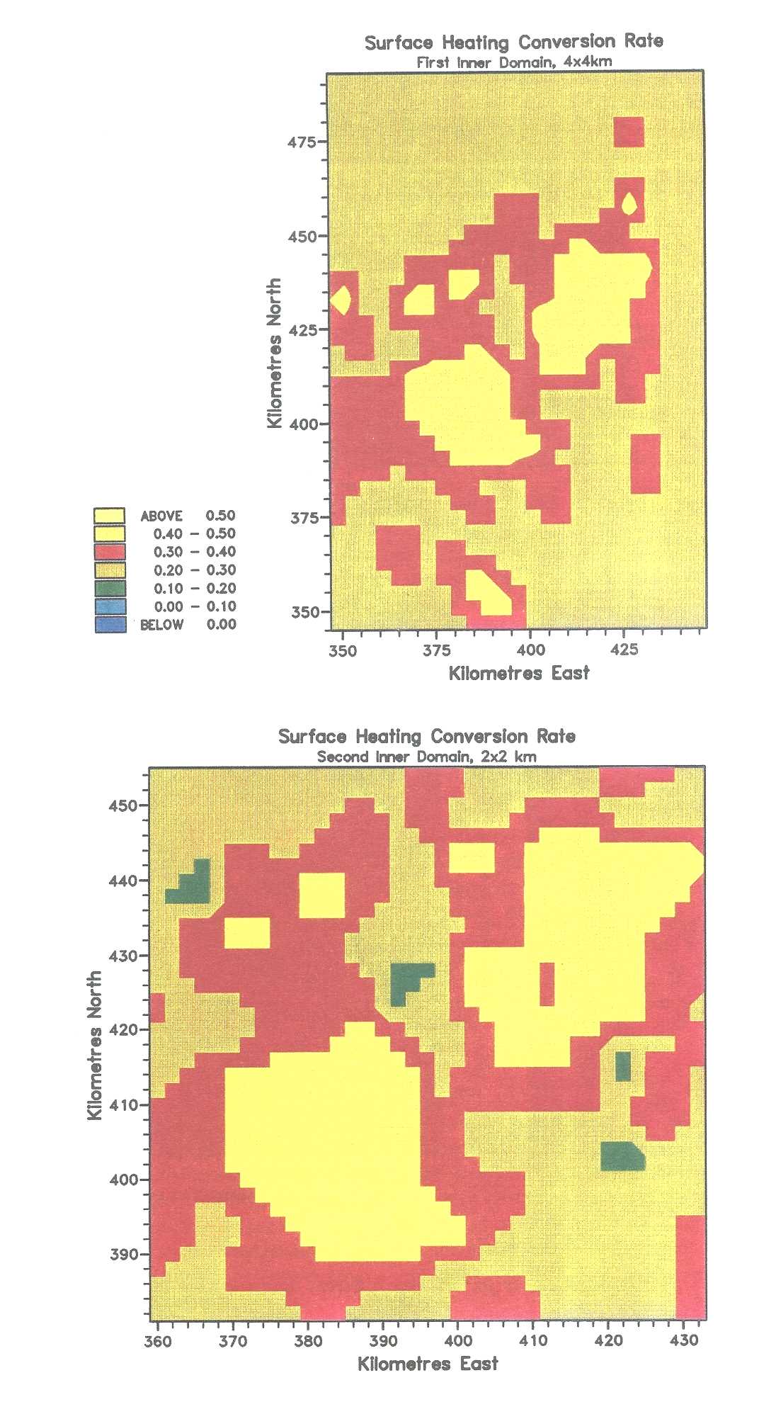
The conversion rate from incoming solar radiation to sensible heat flux μ was also estimated from Ordnance Survey maps. It was assumed that the average conversion rate over land is 30% , but that in case of urban heat island effects cities have a conversion rate of 40%, whereas rivers and lakes only have 20%. In case of no urban heat island simulation the conversion factor was set to 30% throughout the inner domains. In order to simulate converging winds east and west of the Pennines, the conversion rate in the outer domain was set to zero over sea and to 30% over land. This developed a sea breeze effect which then resulted in convergent winds in the two inner domains. If no converging winds were wanted the conversion factor was set equal over sea and over land. The topography of each domain as well as the conversion factor map for incoming solar radiation to sensible heat flux for the two inner domains is shown in Fig. 2 and 3.
In the following 3 model runs are presented. Run FER3DL simulates the outbreak of convection under westerly to southwesterly air flow, without influence of surface wind convergence or urban heat island effects. The numerical results are then compared with radar data (Radar data provided by the Hameldon Hill radar, a conventional C-band weather radar, Plessey type 45C, operating at a wavelength of 5.6cm ) from a storm that developed on the 19th May 1989. The last two model runs simulate convection with mostly southerly winds. Both runs are initiated with the same profiles, but run FER3DJ assumes the presence of urban heat island effects. The numerical results of both runs are compared to convection that broke out on the 24th May.
Run FER3DL was set up with μ=0.3 throughout all domains, thus no surface wind convergence or urban heat island effects were initiated. The temperature and humidity profile used for the simulation was based on meteorological conditions on the 19th May 1989, because observational storm data was available for this time period (Fig. 4). The wind profile was set to 250° from the surface up to 500 hPa, and to northerly veering winds in levels higher than that. The simulations were started at 09:00 GMT in order to give the model time to build up the airflow.
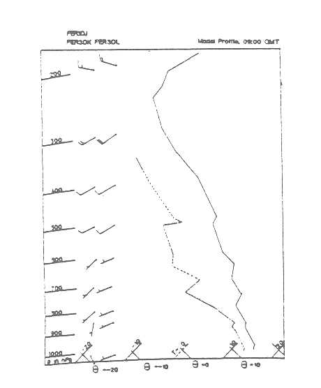
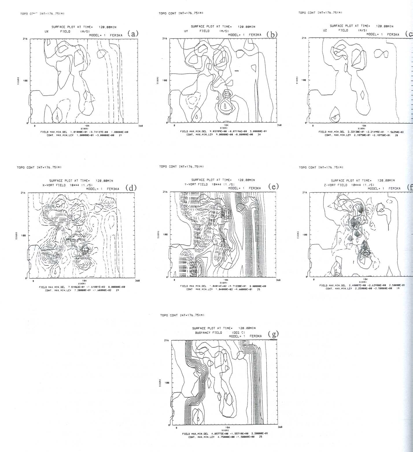
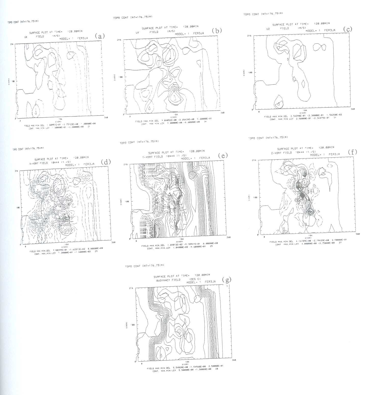
Fig. 5a-g presents the x, y and z components of the wind field (u) and of vorticity (ζ), as well as buoyancy after 120 minutes (=11:00 GMT) of simulation at the surface. Negative values are dashed.
Not surprisingly all three vorticity fields are strongly influenced by the hilly terrain, and steep gradients developed particularly over the ridge of the Pennines. ζx is positive over the hilltops and negative in the valleys, ζy is positive throughout most of the domain, except for a few places where the inflowing air first encounters a valley before rising at the hill slopes. ζx appears to be positive and strongest at the hill tops, whereas in the low lands east and west of the Pennines ζx is predominantly negative.

ux is positive, thus westerly, throughout the domain. It is strongest on the windward side of the ridges where the air is forced to rise and weaker on the leeward side. Because the flow is mainly westerly uy is very weak. However, the hills in the north also force the air to accelerate northwards. uz shows clearly the forced up-draughts at the windward side of the ridges due to forced lifting, and the consequent down-draughts at the east side of the ridges. As expected buoyancy is slightly stronger on the sun-facing eastern slopes than at the western side of the ridges.
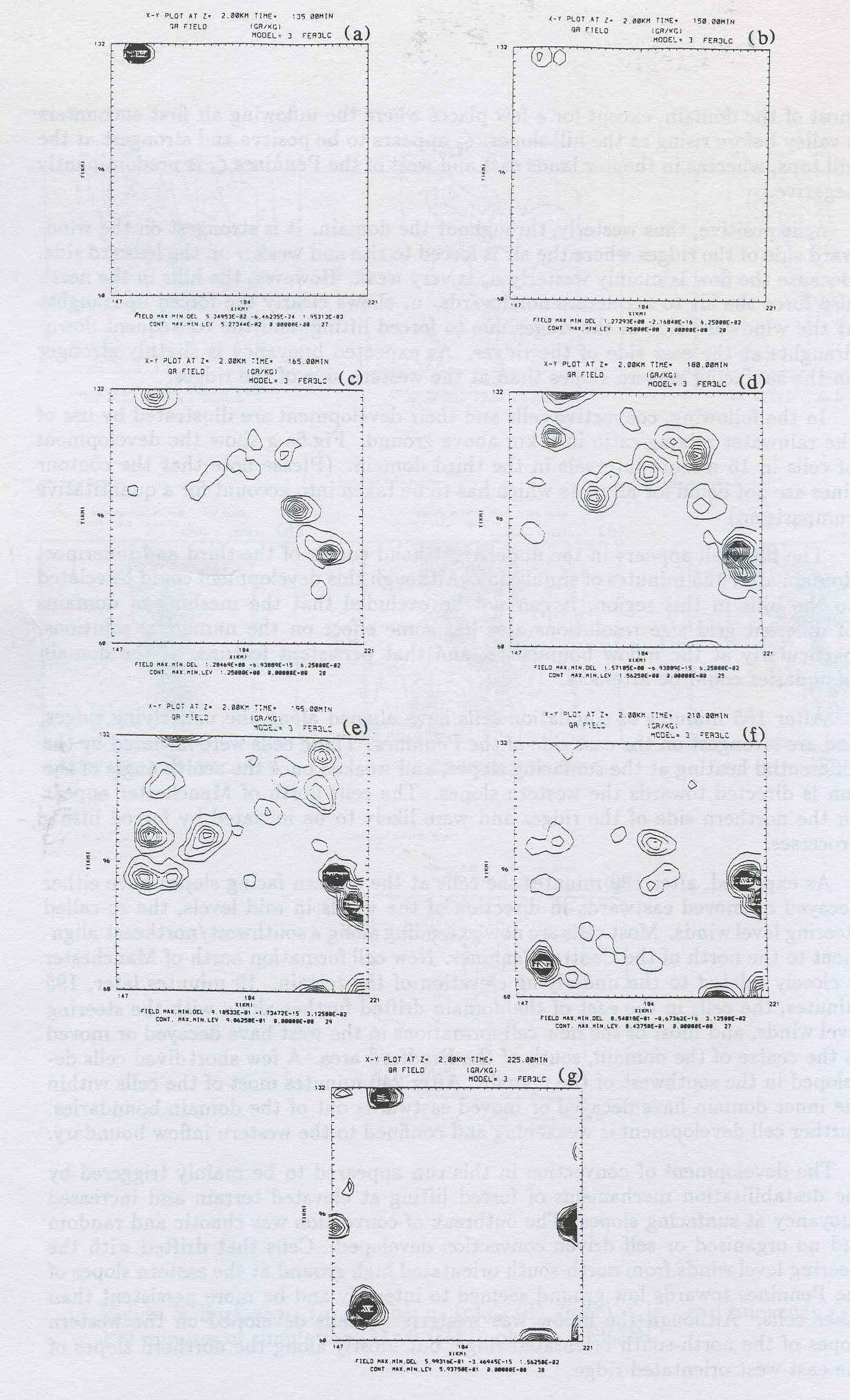
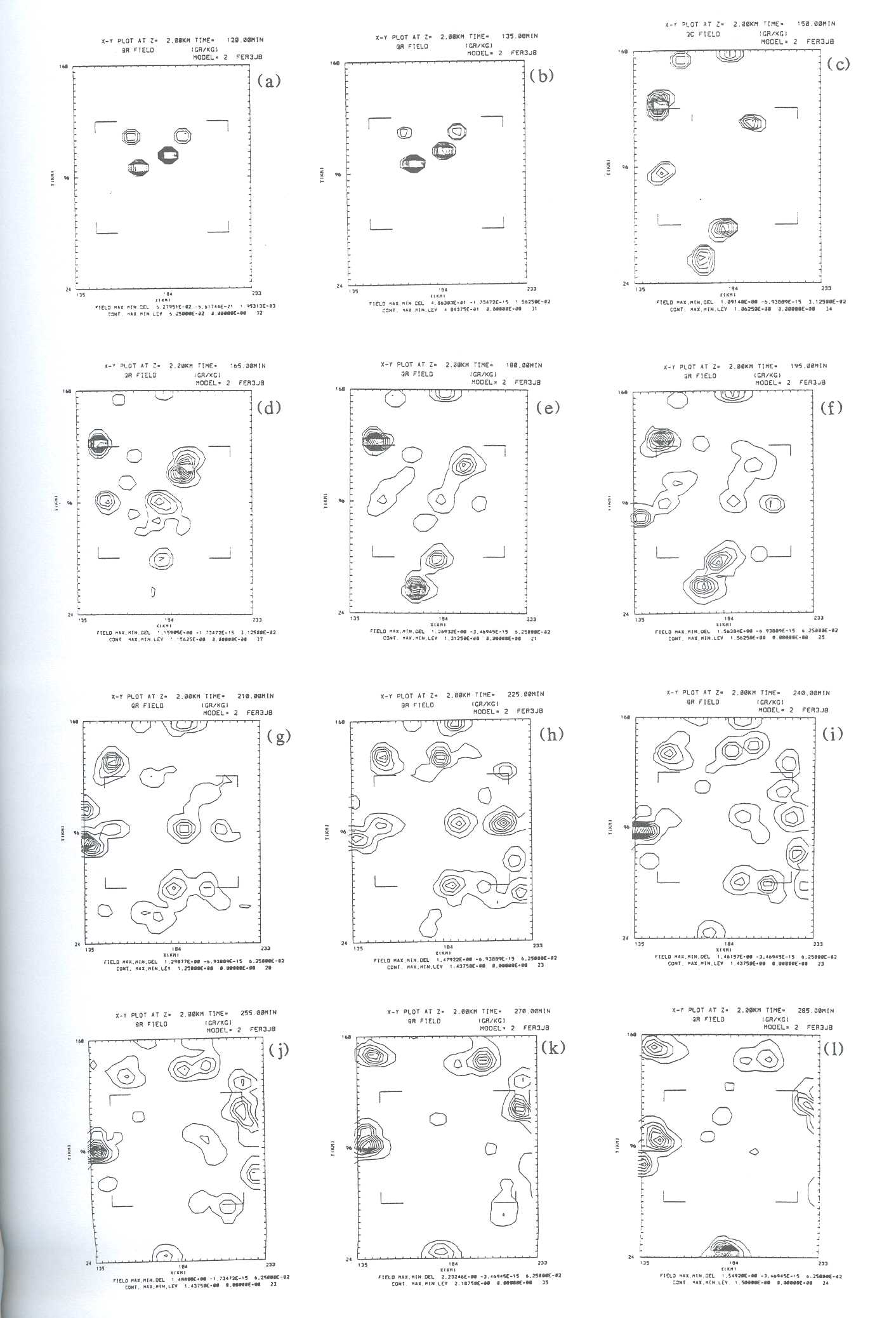
In the following, convective cells and their development are illustrated by use of the rainwater mixing ratio in 2 km above ground. Fig.6a-g show the development of cells in 15 minute intervals in the third domain. (Please note that the contour lines are not equal for all plots which has to be taken into account for a quantitative comparison.)
The first cell appears in the upper right hand corner of the third and innermost domain after 135 minutes of simulation. Although this development could be related to the hills in this region, it can not be excluded that the meshing of domains of different grid size resolutions also has some effect on the numerical solutions, particularly at the inflow boundaries, and that persistent features at the domain boundaries could be artefacts.
After 165 minutes of simulation cells have aligned along the underlying ridges, and are strongest on the east side of the Pennines. These cells were initiated by the differential heating at the sun-facing slopes, and weaken once the zenith angle of the sun is directed towards the western slopes. The cells north of Manchester appear on the northern side of the ridges and were likely to be initiated by forced lifting processes.
As expected, after 180 minutes the cells at the eastern facing slopes have either decayed or moved eastwards in direction of the winds in mid levels, the so-called steering level winds. Most cells are now extending along a southwest/northeast alignment to the north of the Central Pennines. New cell formation north of Manchester is closely related to the underlying elevation of the terrain. 15 minutes later, 195 minutes, the cells in the east of the domain drifted further along with the steering level winds, and most of the new cell formations in the west have decayed or moved to the centre of the domain, south of the Bradford area. A few short-lived cells developed in the southwest of the domain. After 240 minutes most of the cells within the inner domain have decayed or moved eastwards out of the domain boundaries. Further cell development is weakening and confined to the western inflow boundary.
The development of convection in this run appeared to be mainly triggered by the destabilisation mechanisms of forced lifting at elevated terrain and increased buoyancy at sun-facing slopes. The outbreak of convection was chaotic and random and no organised or self driven convection developed. Cells that drifted with the steering level winds from north-south orientated high ground at the eastern slopes of the Pennines towards low ground seemed to intensify and be more persistent than other cells. Although the inflow was westerly no cells developed on the western slopes of the north-south orientated ridge, but mostly along the northern slopes of the east-west orientated ridge.
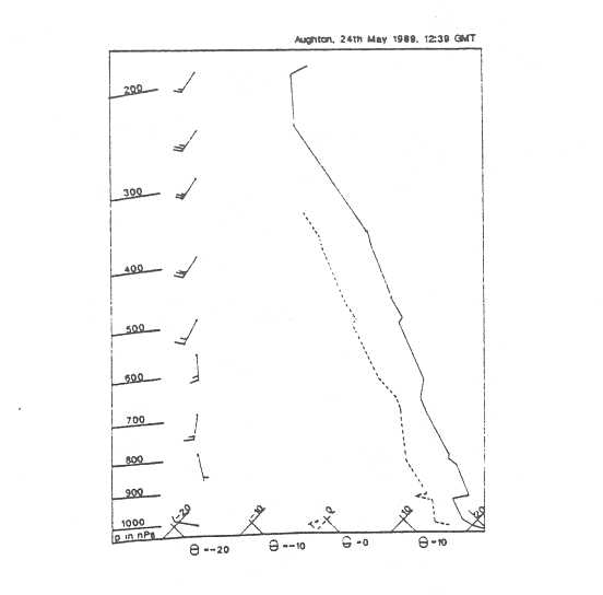
The results of the simulation were compared to a storm that developed on the 19th May 1989 in the Central Pennines, the Halifax storm, which has been addressed in several papers (Acreman 1989, Collinge et al. 1990, Collinge and Acreman 1991, Swann 1993). During the Halifax storm the winds in the steering level were predominantly westerly to southwesterly. The TΦ-gram of the storm as well as the wind profile of the closest radiosonde station upwinds of the storm (Aughton) is given in Fig. 7.
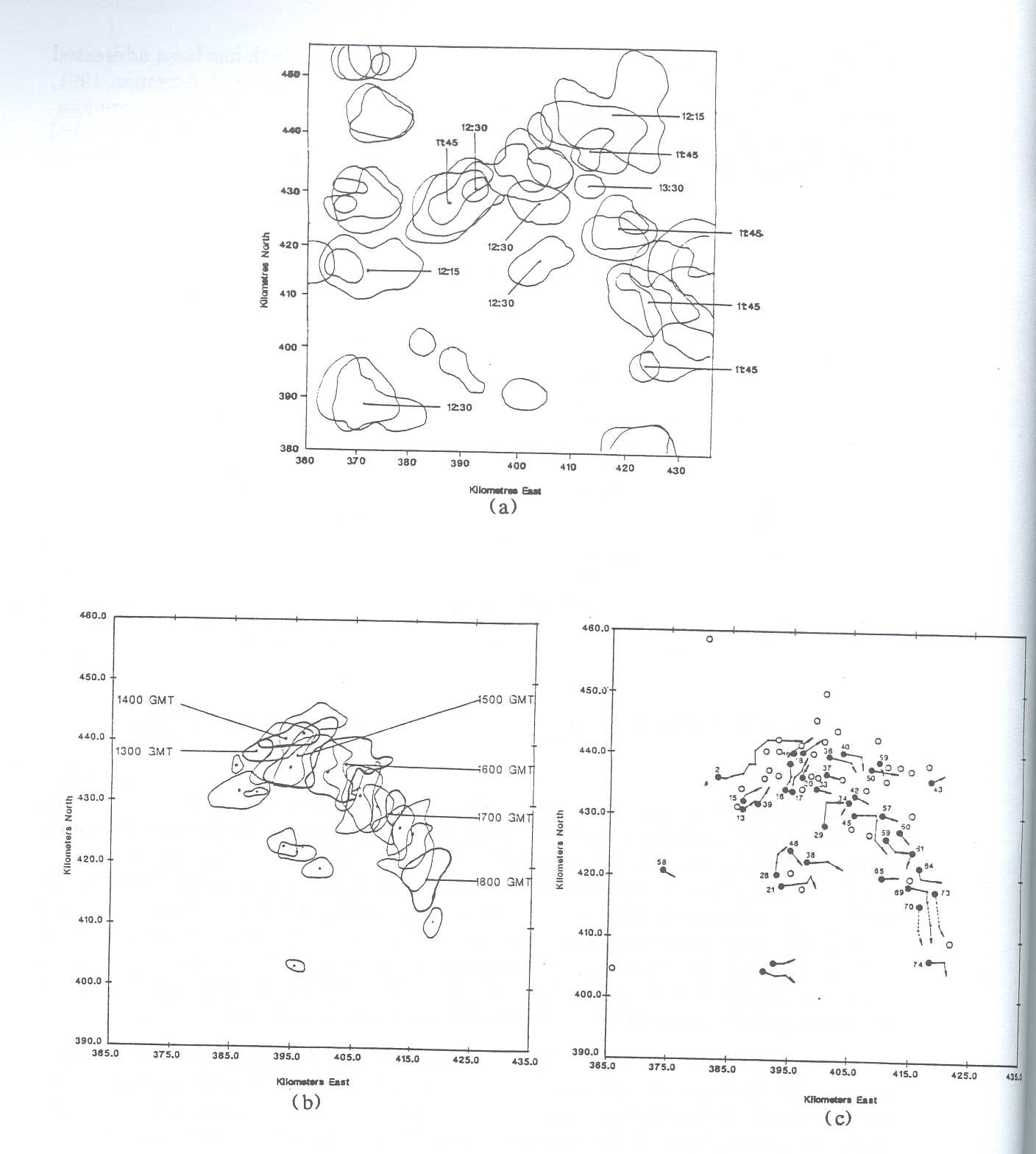
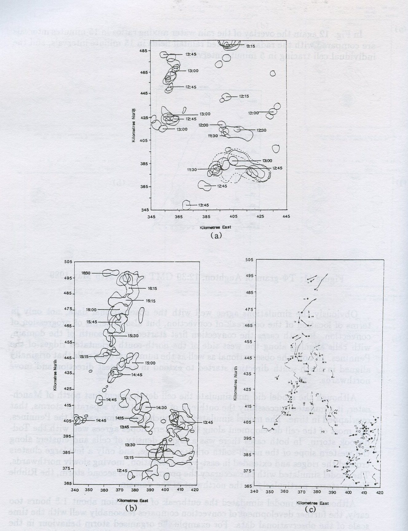
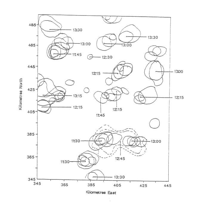
The Halifax storm started off with chaotic and random outbreak of convection along the northern slopes of the east-west orientated ridge of the Central Pennines. After about 2 hours the storm became stationary for about 45 minutes west of Bradford, and then moved on quickly southwards along the eastern slopes of the north-south orientated ridge while intensifying. In Fig. 8 the overlay of contour lines of the radar estimated surface rainfall field in 15 minute intervals are compared with the overlay of the rain water mixing ratio in 2 km height in order to compare the development of convection. For further insight into the observational data the cell tracing in 5-minute intervals of the Halifax storm is also shown.
Apparently there are similarities between the simulation and the Halifax storm, but also some severe differences. In both cases the development of convection seemed closely linked to the underlying topography. In both cases cells developed at the northern slopes of the east-west orientated ridge, and on the eastern slopes of the north-south orientated ridge. No cells developed on the western slopes of the north-south orientated ridge. There was also some independent convection in the corner where the north-south orientated ridge and the east-west orientated ridge are perpendicular.
The cell tracing plot shows that cells during the Halifax storm tended to move with the steering level winds, similarly to the results in the model. The cell tracing also shows that the storm seemed to have split into into two parts, one in which the cells seemed to continue moving northeastwards, while in the other part cells moved southwards along the east side of the north-south orientated ridge. This 'splitting' of convection can also be seen in the model simulations, Further, analysis of the observational data suggested that cells moving from high ground towards low ground were likely to intensify (not shown), which also agrees well with the model results.
However, although the favoured location of cell development seem to be similar between the model results and the simulation, there are severe differences between the development of the actual and model storms. Although in both cases first cells broke out around midday, and developed in a more or less random order along the northern slope of the east-west orientated ridge, there was no outbreak of convection along the eastern slopes of the north-south orientated ridge during the first stages of the Halifax storm. Only after the storm had become stationary around 15:00 GMT, which is indicated in Fig. S8b by the higher density of contour lines in that area, the storm developed into an organised storm with continuous cell formation at its advancing flank. The storm then moved southwards along the ridge, with individual cells passing from its right advancing flank to the left flank where they decayed. During this stage the individual cells intensified which suggests that cells under influence of westerly winds intensify when being directed from high ground of the eastern slopes towards low ground of the east. The model failed to develop both the stationary phase of the storm as well as the organised convection along the eastern slopes during the afternoon. In fact, during later stages the model did not simulate any convection at the eastern slopes. Apparently during the Halifax storm there were other trigger mechanism for convection than just forced lifting and surface heating, which the model did not reproduce. This is also mirrored in the much shorter duration of convection in the model. While the model simulated convection only for about 2 hours, the Halifax storm lasted for 7 hours.
Run FER3DK was set up with the same profiles as FER3DL, except for the wind directions (Fig. 4). It was assumed that there were southerly winds in the lower levels up to 800 hPa, but that the winds in the steering level winds were more westerly. Surface wind convergence was imposed, but no urban heat island effects were considered. During this run the outbreak of convection was not confined to the third domain and therefore the second domain is presented in the following.
The vorticity fields for FER3DK (Fig. 9d-f) differ significantly from FER3DL. ζx is negative throughout the domain with strongest negative (ζx at the windward side just when the air is forced to rise at the ridges. Unlike during run FER3DL the hills of Wales and the Lake District seem to have great influence on ζx on the west coast. Both ζx and ζy are very homogeneous at the east coast. ζy is negative west of the Pennines and west of the welsh mountains, but positive over the ridges and east of the Pennines. However, there is not much difference between the ζz-fields of the two runs, with positive ζz at the hill tops and negative ζz in the lowlands.
The surface wind convergence is evident in Fig. 9a which shows clearly the easterly winds east of the Pennines and westerly winds west of the Pennines. Gradients of Ux are weak just above the Pennines probably due to the convergence zone. Unlike in FER3DL where uy was strongest east of the Pennines, in FER3DK it is strongest west and at the Pennines. The air is accelerating northwards over the hill tops. The air seems to flow around the welsh mountains causing southerly components to the north of the hills. The up-draughts are greatest at the bottom of the hills on the west side of the Pennines, but no down-draughts on the leeward side have developed yet. As expected the buoyancy fields have steep gradients along the coasts where the conversion rate μ steps up from 0% to 30%. Again, buoyancy is slightly stronger at the sun-facing eastern slopes.
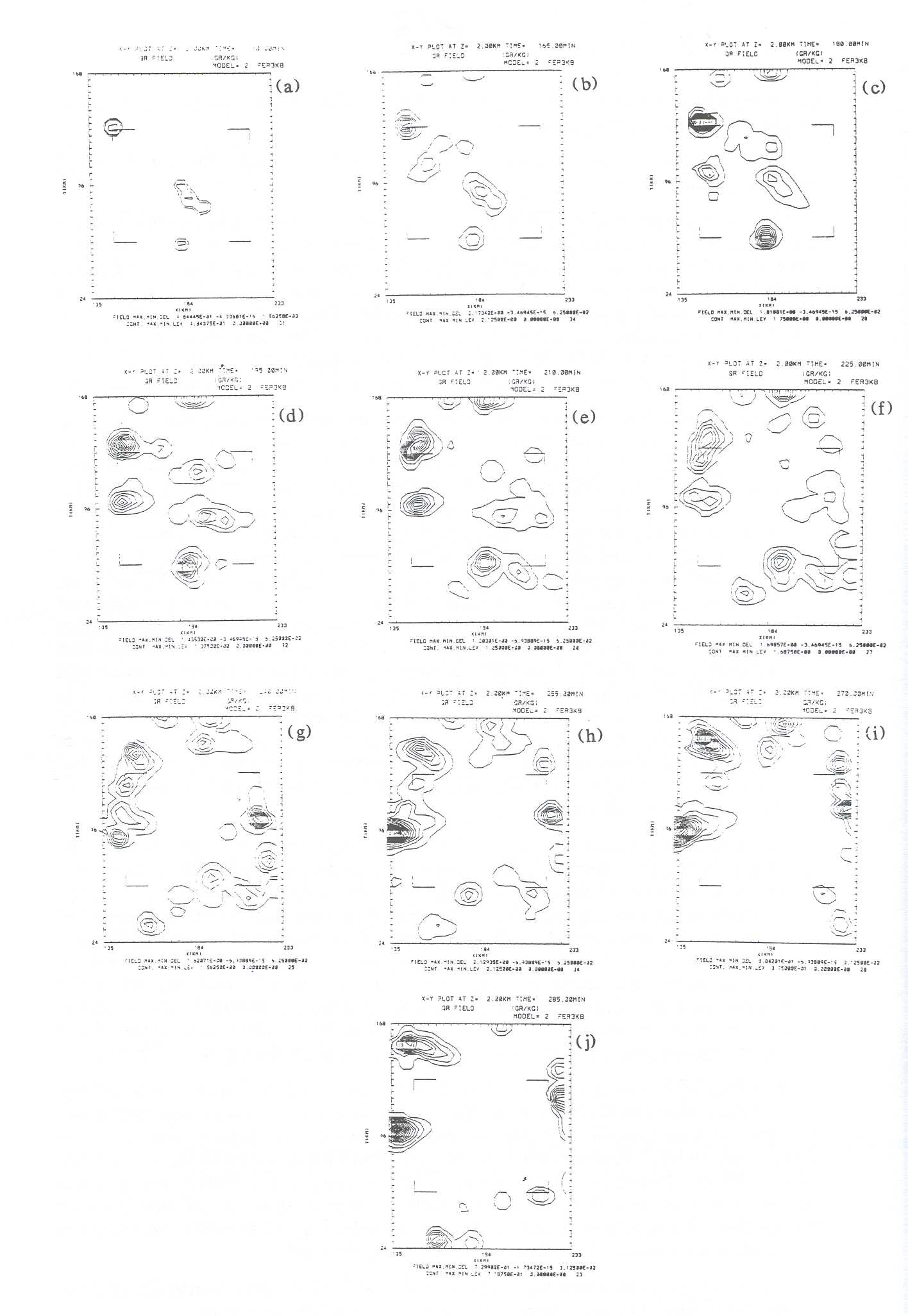
Fig. lOa-j present the development of the rain water mixing ratio in 2 km height in 15 minutes intervals.
Convection started after 135 minutes with first cells starting in the south of the innermost domain at the west side of the ridge. The amount of rainwater however is very little at this stage. It seems that these first cells are initiated by forced lifting at the ridge. 15 minutes later, 150 minutes, convection continues to develop along the western side of the north-south orientated ridge. Similarly to run FER3DL there is convection breaking out at the left upper corner of the innermost domain, and although again this could be due to the underlying topography it seems possible that actual convection is embedded in artefacts due to the meshing of different domains.
After 180 minutes two bands of convection have developed, one along the ridge of the Pennines and one at the western boundary of the inner domain. There seem to be new cells forming in the south of the domain. The cell clusters that were first elongated in north-south directions, following the shape of the underlying ridge, have now extended in east-west direction across the Pennines. These cell clusters continue to move northwards within the next 15 minutes, while similar cell behaviour can be observed in the south of the domain. After 240 minutes of simulation, the separation of the two cell developments becomes more evident. Similarly to run FER3DL cells intensified when moving from the high ground of the eastern slopes of the Pennines towards low ground. While the cells that were confined to the Central Pennines weakened and moved north or eastwards, the convection in the west develops into an elongated band of cells. After 255 minutes of simulation the convection around the Central Pennines have continued to decay, while some new cells developed in the south of the two inner domains. The cells in the west have now intensified and moved northwards, with a light component to the west, thus veering to the left of the steering level winds. Comparison with the underlying topography suggests that the cells in the northwest of the domain move into the valley, which could cause the sudden deviation to the left.
The main destabilisation processes during this run seemed to be forced lifting at hill slopes in the predominant inflow region. Unlike during run FER3DL there was no outbreak of convection in the morning along the sun-facing eastern slopes of the north-south orientated ridges. This is surprising because one could have expected that the easterly surface winds in this region would have enforced the destabilisation process. Convection moved northwards along the underlying ridges, thus with a component to the left of the steering level winds in 700 hPs, and only when the cells were not constrained by underlying elevated terrain individual cells moved in accordance with the winds in 700 hPa. Convection during the second stage of the storm simulation seemed to less random and chaotic than during run FER3DL.
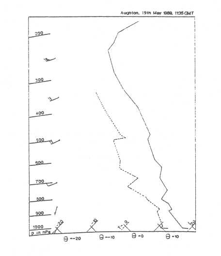
Run FER3DK was compared with the outbreak of convection on the 24th May 1989, 5 days after the Halifax storm. The outbreak of convection on that particular day was wide spread all over Britain and two storms developed in the area, the Toddbrook and the Ribble Valley storm. The Toddbrook storm broke out around 1200 GMT and lasted for about 2 hours. The beginning of the Ribble Valley storm overlapped in time with the end of the Toddbrook storm. It developed northwest of the Toddbrook storm and moved quickly northwards. Fig. 11 presents the TΦ-gram of Aughton on the 24th May 1989 and the upper air winds.
The winds in lower levels up to the steering level winds were southerly, and the surface wind field was convergent towards each side of the Pennines.
In Fig. 12 again the overlay of the rain water mixing ratios in 15 minutes intervals are compared with the radar estimated rainfall fields in 15 minute intervals, and the individual cell tracing in 5 minute interval.
Obviously the simulations agree well with the observational data, not only in terms of location of the outbreak of convection, but also in terms of progression of convection. In both cases the convection first started in the south of the domain, with cells aligning along the west side of the north-south orientated ridges of the Pennines. In both the observational as well as the numerical data cells that originally aligned in north-south direction started to extend in east-west direction and move northwards.
Although the model did not simulate the cell development just north of Manchester, it simulated successfully the outbreak of two spatially separated storms, that overlapped in time. The model simulated too much convection east of the Pennines, but most of the cell development along the western slopes agrees well with the Toddbrook storm. In both cases there was a higher density of cells and clusters along the western slope of the north-south orientated ridge, and only a few large clusters crossed the ridges and extended in east-west orientation, moving slowly northwards. The model simulated with fair accuracy the progress of the second storm, the Ribble Valley storm, particularly in the northwest of the domain.
Although the model simulated the outbreak of convection about 1.5 hours too early, the further development of convection compares reasonably well with the time scale of the observational data. For example the organised storm behaviour in the northwest of the domain lasted both in the simulation as well as in the observations about one hour.
In order to investigate the influence of possible urban heat island effects on the development of convective storms in the Pennines, the same run as FER3DK was performed with the only difference that the conversion rate from incoming solar radiation to sensible heat flux over land was not a constant of 30%, but varied according to Fig. 3. After 120 minutes of simulation, there are hardly any differences in the vorticity or wind fields (Fig. 13a-f). The easterly component of the winds at the eastern slopes of the Pennines are slightly higher than without the urban heat island effects, due to the increased buoyancy over the Manchester and Bradford area (Fig. 13g).
Fig.14a-l show the development of cells in 15 minute intervals in the second domain. Obviously the urban heat island effects force convection to develop about 30 minutes earlier that without heat island effects. First cells appear along the northern slopes of the Central Pennines. After 165 minutes of simulation the results are similar to the ones of run FER3DK, except for strong cell convection in the area of Bradford, and slightly stronger convection south of the Manchester area. Overall convection seemed to align more in a southwest-northeast direction than in the FER3DK run. The development of convection east of the Pennines is stronger and more wide spread than without urban heat islands. Comparison with the observational data shows that during the morning the inclusion of the urban heat island effect seem to worsen the results of the simulation, whereas it seems to improve them during the afternoon (Fig. 15). This is conclusive with results from Oke (1978) which found that urban heat island effects only develop during the afternoon and are greatest during evenings and nights.
The model simulations as well as the investigations of the observational data suggest that the outbreak of convection is very closely related to the winds in the lower levels up to the steering level winds, but that the actual surface winds do not play an important role.
Westerly winds seem to favour the outbreak of convection along the northern slopes of the east-west orientated ridges, thus along an imaginary line from Blackburn to Harrogate. Under influence of westerly winds in lower levels the outbreak of convection along the eastern slopes of the north-south orientated ridges are likely before noon when the slopes are exposed to direct sunlight. However, later during the day outbreak of convection is not likely along the eastern slopes, unless the convection is organised by some self-driven mechanism. Most of the convection then seems to develop along the western slopes.
Southerly winds up to the steering level seem to favour the initiation of convection west of the Pennines. The outbreak and movement of cells seem to be very closely related to the underlying ridges. All cells tended to move northwards, and particularly the valley north of Blackburn and Burnley seem to be favourable for the outbreak of strong convection when under influence of southerly winds.
A could be expected from theory urban heat island effects only seem to improve results during afternoon simulations. Under influence of southerly winds urban heat island effects seemed to favour the outbreak of convection in the area of Bradford and south of Manchester. It can therefore be assumed that storms that break out during the afternoon under influence of southerly winds favour the development of fairly stationary convection in the Bradford area.
The results presented above have shown that the model used for this study is a powerful tool to investigate the influence of the Pennines on the development of storms in the area. The model reproduced convective development on the 24th May 1989 with great detail in terms of outbreak of location of cells, cell movement, and cell development. Although the model failed to simulate the temporal progress of the Halifax storm on the 19th May, it succeeded in calculating the favourable locations of cell outbreaks.
Acreman M. (1989) Extreme rainfall at Calderdale, 19 May 1989; Weather, Vol. 44, pp 438-446
Clark T.L. (1977) A small-scale dynamic model using a terrain-following coordinate transformation; J.Comp.Phys., 24, pp 186-215
Clark T.L. (1979) Numerical simulations with a three-dimensional cloud model: lateral boundary condition experiments and multi-cellular severe storm calculations; J .Atmos.Sci., 34, pp 2191-2215
Clark T.L. and Hall W.D. (1991) Multi-Domain Simulations of the Time Dependent Navier-Stokes Equations: Benchmark Error Analysis of Some Nesting Procedures. J. Comp. Phys., 92, No. 2, pp 456-481.
Clark T. and Farley D. (1984) Severe Downslope Windstorm Calculations in tow and three spatial dimensions using anelastic grid interactive grid nesting: a possible mechanism for gustiness; J.Atmos.Sci., 41, pp 329-350
Collinge V.K. and Acreman M. (1991) The Calderdale storm revised: an assessment of the evidence; BHS 3rd National Hydrology Symposium, Southampton
Collinge V.K, Archibald E.J., Brown K.R. and Lord M.E (1990) Radar observations of the Halifax storm, 19 May 1989; Weather, Vol. 45, No. 10
Koenig and Murray (1976) Ice-bearing cumulus cloud evolution, Numerical simulation and general comparison against observation; J .Appl.Met., 15, pp 747-762
Ogura Y. and Phillips A (1962) Scale analysis of deep and shallow convection in the atmosphere; J Atm.Sci., 19, pp 173-179.
Oke T.R. (1978) Boundary Layer Climates; Methuen & Co .. Ltd, London
Reynolds G. (1978) Maximum precipitation in Great Britain; Weather, May 1978, Vol. 33, No. 5, pp. 162-166
Smolarkiewicz P.K. and Clark T.L. (1985) Numerical simulation of the evolution of a three-dimensional field of cumulus clouds, Part I: Model description, comparison with observations and sensitivity studies; Journ. Atm. Sci., Vol. 42 (5), pp. 502-522
Swann H. (1993) Modeling convective systems on the large eddy simulation model; Internal Report, Joint Centre for Mesoscale Meteorology, Newsletter No. 4, Feb 1993
I would like to acknowledge the support of Dr. A. Gadian and R. Lord who have helped me to understand the model and to overcome the numerous problems associated with the code. I would like to thank Dr. T. L. Clark and Dr. W. Hall for information, advice and help with the latest version of the code, and also Dr. J. F. R. Mcilveen who has spend valuable time discussing both observational and model results with me. Financial support for this study was given by the SERC (GR9/814) and the EC (CEC 900898). I would also like to thank the user support group of the RAL for helping to solve problems related to the use of the CRAY.
The Atlantic Ocean is important because of its influence on the world's climate. Warm near-surface waters flow northwards and release their heat to the atmosphere in the wintertime at high northern latitudes. This results in sinking and the production of deep cold return flows to the south. The whole process has been dubbed the "Atlantic Conveyor Belt" and is responsible for a large heat exchange to the atmosphere. It is therefore important to understand the processes which contribute to the heat transport and circulation in the Atlantic.
Isopycnic-coordinate models, consisting of a set of layers of constant density but varying thicknesses, are now emerging as a useful tool for the investigation of these ocean processes. These models are in contrast to the more usual gridpoint models which have a set of levels at fixed positions in the vertical at which the model variables are known, and which have been in use for many years. Isopycnic models may possess certain advantages over the gridpoint models, but so far most ocean modelling studies and climate prediction models have been based around the gridpoint models.
It is therefore important to intercompare these two model types to assess their relative merits. With this in mind, the James Rennell Centre for Ocean Circulation have implemented the Miami isopycnic model to describe the Atlantic Ocean from about 15°S to 80°N, and a 30-year integration has been carried out at a relatively low resolution of, nominally, 1° horizontally (latitude-longitude). As a collaborative exercise, the Hadley Centre for Climate Prediction and Research (part of the UK Met. Office) has carried out a parallel integration with a gridpoint model, and significant differences are now emerging. In particular, the overall heat carried northwards differs by more than 50% between the two models, and there are significant differences in the outflows of deep water masses across the Greenland-Iceland-Faeroes rise, and in the path of the North Atlantic Current. These discrepancies are likely to cause large differences in climate models which may be integrated for long periods, but it is still too early to say precisely what causes the differences, although further study is in progress. The low resolution isopycnic model is also giving significant insights into the interdecadal variability of the subtropical gyre, and has been compared with observations to good effect, and is also showing the significance of an accurate representation of the Gulf Stream.
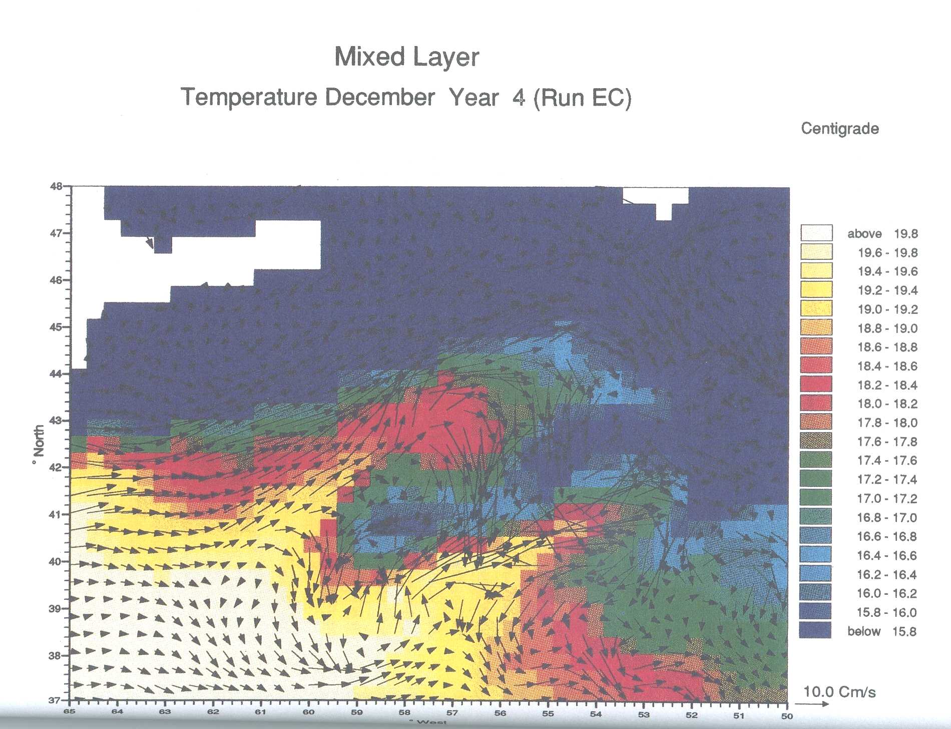
The model is now also being run at a higher horizontal resolution, about 1/3°, which is sufficient to allow eddies to form. Eddies are the weather systems of the ocean, and usually occur on scales of 20-200km or thereabouts. As such, they are too small to be adequately described by typical climate models, which for reasons of computer size and speed, usually have a resolution of 1° or 2° horizontally. Nevertheless, it may be that these eddies contribute significantly to the basin-averaged northward heat transport and also to the interactions and transfers between the ocean surf ace and its interior. It is therefore necessary to perform model integrations containing eddies so that these effects can be studied and, if found to be important, so that parameterisations can be developed for inclusion in the climate models. Several initial tests with the Miami code have now been undertaken on the RAL CRAY YMP. Work has so far concentrated on varying the available parameters to obtain a realistic eddy field. Although further tests are still required, it has already been possible to obtain realistic eddies in certain cases. As in the real world, a cyclonic (anti-clockwise) cold-core eddy has been observed south of the mean position of the core of the Gulf Stream, with a corresponding anticyclonic warm-core feature to the north. This is shown in the figure, which reveals the sea-surface temperature and current structure in one of the eddy-resolving runs just south of Nova Scotia (the cold-core eddy occurs at 58°W, 41°N, the warm eddy at 57°W, 43°N). The net effect of these eddies must be to increase the northward heat transport, at least locally across the Gulf Stream, since cold water from north of the current is being drawn southwards, to form the cold-core feature, and conversely for the warm feature. Collaboration is now beginning with similar modelling groups in Germany and France to intercompare three different model types at eddy resolution, in order to assess their relative merits.
New, A. L. 1991a. Atlantic Isopycnic Model. p 5 in Sigma, The UK WOCE newsletter, number 4, May 1991.
New, A. L. 1991b. Atlantic Isopycnic Model (AIM) - current status. p 2 in Sigma, the UK WOCE newsletter, number 5, September 1991.
Barnard, S. Y. Jia and A. L. New, 1992. A study of Labrador Sea Water in the Atlantic Isopynic Model. Proc. Challenger Soc. conference "UK Oceanography 1992", Liverpool 21-25 September 1992. (Abstract only.)
Marsh, R. and A. L. New, 1992. The Atlantic Isopynic Model, AIM: progress and plans. Sigma, the UK WOCE newsletter, no.7, 4-6.
New, A. L. 1992. The Atlantic Isopynic Model: AIM. Proc. Environmental Sciences Seminar "The power in your predictions", Utrecht, Holland, 22 October, 1992, organised by CRAY Research B.V. Rijswijk, Holland. 14pp.
New, A. L. R. Bleck, Y. Jia, R. Marsh, S. Barnard and M. Huddleston, 1992. A simulation of the Atlantic Ocean with an isopycniccoordinate circulation model. Proc. Challenger Soc. conference "UK Oceanography 1992", Liverpool 21-25 September 1992. (Abstract only.)
New, A. L. Y.Jia, R. Marsh, S. Barnard, M. Huddleston and R. Bleck, 1992. An isopycnic model of the North Atlantic Ocean. Annales Geophysicae, supplement II to volume 10, p 179 (abstract only). 248pp.
Nurser, G. and R. Marsh, 1992. Subduction and buoyancy forcing in the Atlantic Isopycnic Model. Sigma, the UK WOCE newsletter, no. 8, 10-11
Barnard, S. Y.Jia and A. L. New, 1993. Labrador Sea Water in the Atlantic Isopycnic Model (AIM). Sigma, the UK WOCE newsletter, no. 9, 8-9.
When the purchase of a Cray X-MP was announced by ABRC in 1986, the NERC Ocean modelling community put forward a proposal to make a significant advance in modelling the ocean. The resulting project, FRAM, produced the first high resolution model of the Southern Ocean. The Southern Ocean was chosen as an important, yet relatively unstudied region, whose physics is very different from that of other ocean basins, primarily because of the lack of eastern and western boundaries. The Antarctic Circumpolar Current (ACC), which dominates the Southern Ocean, provides an important connecting link transporting and mixing water masses between the other major oceans of the world. It also acts as a barrier to the transport of heat by the ocean between the tropics and Antarctica.
The main FRAM run started on the Cray X-MP at the Atlas Centre, Rutherford Appleton Laboratory, in the spring of 1989 and ended in April 1991. A total of 16 model years was completed. Following this, two-and-a-half model years was completed of a second run, which included a sea-ice model This model was transferred to the CRAY Y-MP.
The model results were very realistic. They showed that the ACC had a large scale braided structure with localised, very strong barotropic flows associated with sharp topographic features. Some unexpected features, such as strong, narrow jets flowing through the fracture zones of the South Pacific, were also evident. These have since been confirmed by observation.
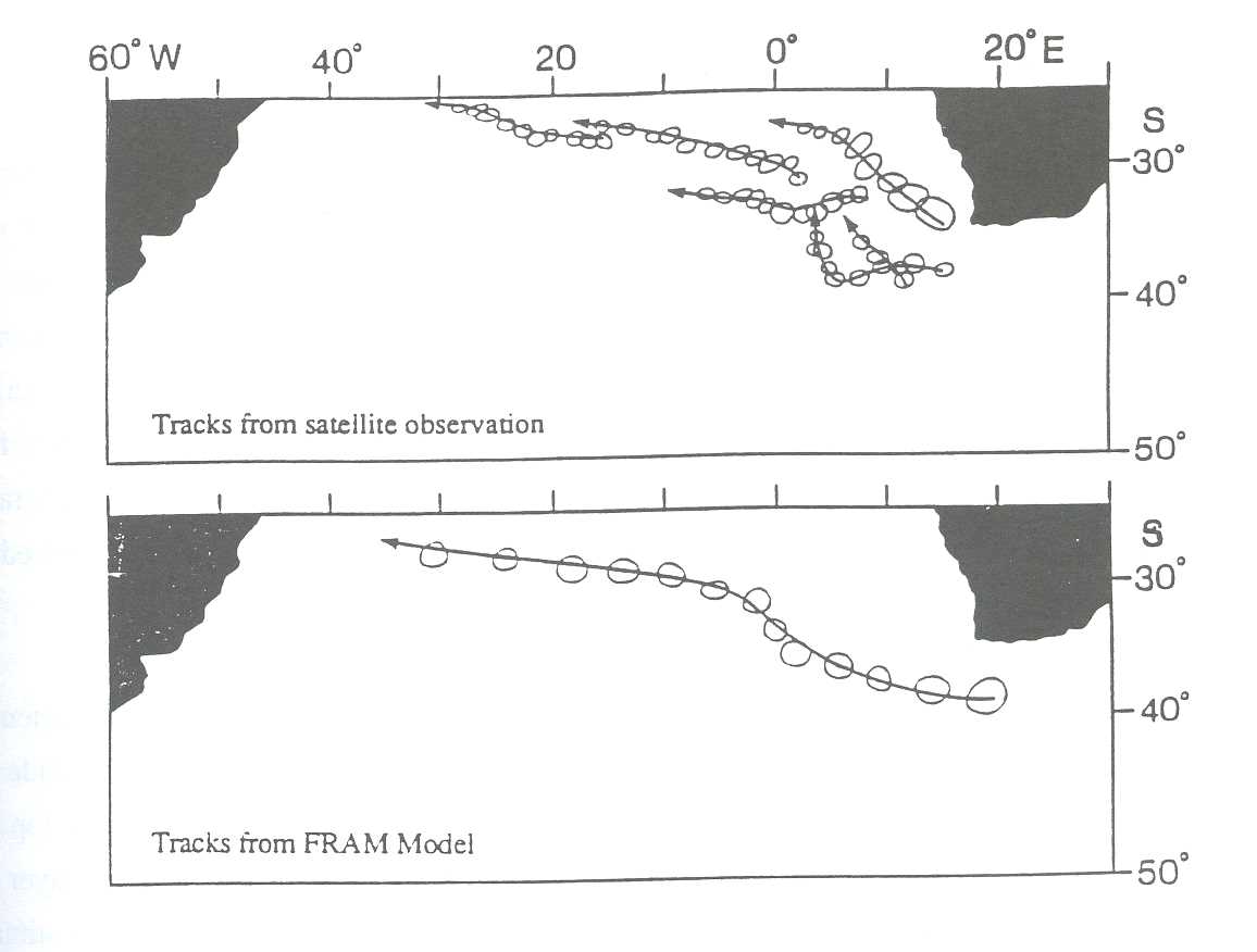
Although the Levitus historical data used to initialise the model do not show sharp fronts, the model dynamics proved very effective at sharpening up the temperature gradients to produce fronts. In Drake Passage, for example, the model shows the ACC to consist of three fronts, in agreement with hydrographic and current measurements in the region. South of Africa the model produced a strong Agulhas Current and a realistic re-circulation zone. Eddies are generated in this region and are shown by the model to drift slowly north-westward into the South Atlantic (Figure 1). Comparisons between model results and satellite data in this region confirm that the strength of the currents is realistic, but that the model re-circulation zone is slightly further east than it should be. This appears to be related to the smoothing applied to the model topography.
The results from the FRAM model were published in the form of an atlas which illustrated the model state at the end of the six year spin-up period. Over 400 copies have been distributed worldwide. As a result, FRAM data have been supplied to researchers in Europe, North America, South Africa and Australia. A video was produced in collaboration with the Atlas Centre of time series of the model fields in key areas. This has been used as a research tool and at international seminars.
FRAM was a NERC Community Research Project and much important analysis of the model has been undertaken at IOSDL and the Universities of East Anglia, Southampton, London (Imperial College and University College), Oxford, Cambridge and Exeter. This analysis is still continuing. Three areas will be highlighted here.
Dr D Stevens (UEA) and Dr V Ivchenko (Southampton University) studied the momentum balance of the ACC. They found that at the latitudes of Drake Passage, the surface wind stress is balanced by the northward Ekman transport and that this is lost to the Deacon Cell (see (iii) below) return flow region below 2000 m. They also looked at the zonal momentum balance, where, in addition to the balances above, they found that in the top 2000 m, the Coriolis term is balanced by the eddy Reynolds stress. Standing eddies (departures from zonal flow of the mean current) make the largest contribution to this balance. Integrating around Antarctica, the standing eddies act as a drag on the ACC but the transient eddies cause a small acceleration of the flow.
Dr P Killworth and Dr M Nanneh of the Hooke Institute, Oxford, studied the momentum balance in the Southern Ocean working on density surfaces and averaging in longitude and time. They found the momentum balance in each layer to be primarily between top and bottom form stress. In some of the deep layers the mean north-south flow in the layer is a result of a long term thermohaline response of the model to the initial conditions. Estimates indicate that this would take about 200 years to empty or fill a layer, which is comparable to the flushing time of the ACC area. These results are important in that they show that the 16 year run of the FRAM model is not in dynamical equilibrium. This will be true of most other models in which long term changes in the thermohaline circulation induce Coriolis forces, which in turn require bottom pressure torques to balance them.
Dr P Saunders and Mr S Thompson of IOSDL have studied the heat transport in FRAM. They have found the net heat transport to be southwards at all latitudes. North of 35°S the heat is carried primarily by the mean circulation. In the South Atlantic this is dominated by the thermohaline circulation, but in the other oceans it is dominated by the gyre scale circulation. Opposing this southwards transport is a strong northwards heat transport due to the surface Ekman layer. Near 40°S, at the latitude of the Agulhas retroflection region, the heat transport by the mean current field is northwards and the main southward heat transport is due entirely to the fluctuations in the flow. These continue to be important north of 60°S, but further south the mean circulation again dominates. This is an important result as it is the first time that the eddy field has been found to dominate the heat transport in a large scale ocean model. As studies of other regions of the world ocean have failed to find such behaviour, the Southern Ocean between 30°S and 60°S may be the only region of ocean in which the fluctuations are responsible for a significant fraction of the heat transport.
Dr K Doos of IOSDL has studied the meridional circulation of the Southern Ocean. A key component of this circulation is the Deacon Cell, consisting of the northward driven water in the surface Ekman layer and the Ekman return flow which occurs at depths of 1500 m and more. This cell shows up strongly in the coupled ocean-atmosphere models used for climate studies and in the past has appeared responsible for the slow response of the Southern Ocean to climate change. By studying the circulation using averages made on both depth and density co-ordinates, Dr Doos has shown that the Deacon Cell circulation does not involve any changes in density. Instead, as a study with Dr D Webb has shown, the Deacon Cell is composed of a large number of overlapping small cells in which the water particles each only move vertically a few hundred metres. At intermediate depths, less dense water is able to transfer momentum coming from the wind to denser water masses, which in tum carry it lower in the water column. In this way the surface wind stress is carried down to depths where the return flow in the Deacon Cell can lose it in topographic form drag.
On the basis of the insight obtained from the model data, Dr Doos has developed an analytic model which shows how the Deacon Cell develops in the gyre regions away from the latitudes of Drake Passage. Independently, Dr Webb has used the results to develop a separate theory of how the Deacon Cell return flow crosses the latitudes of Drake Passage as a deep western boundary current attached to the Kerguelen Plateau. Previous theories had always failed to explain this part of the circulation.
The running and analysis of FRAM has produced an order of magnitude increase in our understanding of how the ACC works. It has also taught the UK modelling community how to run very large models of the ocean and how to handle the huge amounts of data that such models produce. The problems of the limitations of present models and the areas in which improvements are needed for future climate research are being tackled as part of the new OCCAM (Ocean Circulation and Climate Advanced Modelling) Community Research Project.
Gordon, A.L. & W.F. Haxby, 1990. Agulhas Eddies invade the South Atlantic: Evidence from Geosat altimeter and shipboard conductivity-temperature-depth survey. J. Geophys. Res. 95, 3117-3125.
A R Clare & D P Stevens Implementing finite difference ocean circulation models on MIMD, distributed memory computers. Future Generation Computer Systems, 9 (1993), 11-18.
H L Jones & J C Marshall Convection with rotation in a neutral ocean; a study of open-ocean deep convection. Journal of Physical Oceanography, 23 (1993), 1009-1039.
P D Killworth An equivalent-barotropic mode in the Fine Resolution Model. Journal of Physical Oceanography, 22 (1992), 1379-1387.
PD Killworth, D Stainforth, DJ Webb & SM Paterson The development of a free-surface Bryan-Cox-Semtner ocean model. Journal of Physical Oceanography, 21 (1991), 1333-1348.
J RE Lutjeharms, DJ Webb & BA de Cuevas Applying the Fine Resolution Antarctic Model (FRAM) to the ocean circulation around Southern Africa. South African Journal of Science, 87 (1991), 346-349.
J R E Lutjeharms, F A Shillington & C M Duncombe Rae Observations of extreme upwelling filaments in the southeast Atlantic Ocean. Science, 253 (1991), 774-776.
J C Marshall, D Olbers, H Ross & W Gladrow Potential vorticity constraints on the dynamics and hydrography of the Southern Ocean. Journal of Physical Oceanography, 23 (1993), 3,465 - 487
P Saunders & S R Thompson Transport, heat and freshwater fluxes within a diagnostic numerical model (FRAM). Journal of Physical Oceanography, 23 (1993), 452-464.
G A Schmidt & E R Johnson Direct calculation of low-frequency coastally-trapped waves and their scattering. Journal of Atmospheric and Oceanic Technology, 10 (1993), 368-380.
D P Stevens The open boundary condition in the United Kingdom Fine Resolution Antarctic Model. Journal of Physical Oceanography, 21(1991), 1494-99.
D P Stevens & PD Killworth The distribution of kinetic energy in the Southern Ocean. A comparison between observations and an eddy-resolving general circulation model. Philisophical Transactions of the Royal Society, B, 338 (1992), 251-257.
The FRAM Group (D J Webb et al) An Eddy-resolving model of the Southern Ocean. EOS, Transactions of the American Geophysical Union, 72 (1991), 169-174.
D J Webb A simple model of the effect of the Kerguelen Plateau on the strength of the Antarctic Circumpolar Current. Geophys. Astrophys. Fluid Dynamics, 70 (1993), 57-84.
D G Wright & A J Willmott Buoyancy driven abyssal circulation of the Southern Ocean. Journal of Physical Oceanography, 22(1992), 139-155
A R Clare & D P Stevens Porting a finite difference ocean circulation model to the Meiko computing surface. In: Proceedings of the International Conference on Parallel Computing '91. Elsevier, pp 585-592. ( 1992)
A C Coward The equation of state algorithms used by the OCCAM model. Institute of Oceanographic Sciences, Internal Document No. 323 (1993).
A C Coward & B A de Cuevas The FRAM Atlas of the Southern Ocean. NERC News, January 1992.
B A de Cuevas The main runs and datasets of the Fine Resolution Antarctic Model Project (FRAM). Part I: The coarse resolution runs. Institute of Oceanographic Sciences, Internal Document No. 315 (1992). 39pp.
B A de Cuevas The main runs and datasets of the Fine Resolution Antarctic Model Project (FRAM). Part II: The data extraction routines. Institute of Oceanographic Sciences, Internal Document No. 319 (1993). 61pp
T Hateley & B A de Cuevas The main runs and datasets of the Fine Resolution Antarctic Model Project (FRAM). Part III: The data extraction routines. Institute of Oceanographic Sciences, Internal Document No. 319 (1992). 61pp
N P Plummer DBDB5 data set of global bathymetry Institute of Oceanographic Sciences Internal Document, No. 300 (1991). 36pp.
G A Schmidt & E R Johnson Grid dependence in the numerical determination of topographic waves. Ocean Modelling, 99 (1993 ), 10-11.
H M Snaith Technical Note : A simple iterative method to improve geosat along track sea surface height data. International Journal of Remote Sensing, 14 (1993), 1715-1722.
H M Snaith & D J Webb Comparisons of ERS-1 altimeter height data and the Fine Resolution Antarctic Model (FRAM). pp. 141-146 in, Space at the service of the environment: Proceedings of the 1st ERS-1 Symposium, Cannes, 4-6 November 1992. Paris: European Space Agency (1993). (ESA SP-359)
D J Webb FRAM - The Fine Resolution Antarctic Model. In: Computer Modelling in the Environmental Sciences. Institute of Mathematics and its Applications. ( 1991)
D J Webb The Fine Resolution Antarctic Model. NERC News 14 (1991), 28-31.
D J Webb Results from FRAM - The Fine Resolution Antarctic Model. Proceedings of the GLOBEC Workshop on Southern Ocean Zooplankton and Climate Change. (Held May 1991, La Jolla, USA)
D J Webb The equation of state algorithms used by the FRAM model. Institute of Oceanographic Sciences Internal Document, No. 313 (1992). 34pp.
D J Webb Contributory author to 'Climate modelling, climate prediction and model validation'. (Lead authors: W.L. Gates, J.F.B. Mitchell, G.J. Boer, U. Cubash, & V.P. Meleshko.) pp 97-134 (section B) of 'Climate Change 1991, The Supplementary Report to the IPCC Scientific Assessment'. Eds: J.T. Houghton, B.A. Callaner & S.K. Varney. (1992)
D J Webb FRAM - the Fine Resolution Antarctic Model. pp. 314-317 in, Fourth International Conference on Southern Hemisphere Meteorology and Oceanography, March 29 - April 2 1993, Hobart, Australia. Boston, MA: America! Meteorological Society (1993). 533pp.
D J Webb An ocean model code for array processor computers. Institute of Oceanographic Sciences Internal Document, No. 324 (1993). 21 pp.
D J Webb, P D Killworth, AC Coward & SR Thompson The FRAM Atlas of the Southern Ocean. Natural Environment Research Council, Swindon (1991). 67pp.
M White Current meters in FRAM - Data Report. Department of oceanography, University of Southampton Data Report .. SUDO/TEC/91/7 NC. April 1991.
A dynamically coupled model for wind wave and storm surge prediction has been developed at Proudman Oceanographic Laboratory. This model, consisting of a third generation wave model (WAM) coupled to a barotropic tide/surge model, considers various interactions between tides, surges and waves. It is anticipated that the fully coupled model will give better forecasts of waves as well as sea surface elevations and currents than the separate models presently in use.
Among the wave and tide/surge interactions examined at early stages of the project, the influence of changes of water levels and currents on the propagation of waves and the influence of wave-dependent surface and bottom stresses on tide/surge generation, propagation and dissipation have been found to be most significant in shelf sea models. Idealised cases were studied in order to establish a depth and current refraction scheme incorporated in the WAM model. In particular, the influence of directional resolution on wave refraction was examined, together with its computational costs.
The coupled wave-tide-surge model has been used to simulate real storm events in the Northwest European continental shelf seas. It was implemented on a large scale grid covering NW European shelf with resolution of 1/3° in latitude by 1/2° in longitude, as well as on a finer grid (resolution 1/9° in latitude by 1/6° in longitude; approximately 12Km) nested within it and covering the English Channel and the Irish Sea.
An example is shown in Figures 1-2 of the interaction of waves with tides and surges during the storm of 26 - 27 February 1990, which breached a sea wall at Towyn in North Wales and caused serious flooding with about 2000 people evacuated from their homes. Fig. 1 shows the difference in modelled significant wave height at 11z on 26th February caused by time-varying depth and current due to the presence of tides and storm surges, while Fig.2 shows the computed change in sea level at the same time caused by wave-dependent surface and bottom stress. It can be seen that both changes in local wave height and sea level are significant, particularly in coastal areas where they exceed lm in wave height and 0.75m in sea level. This also demonstrates a need for even better resolution models (requiring even more supercomputing resources) covering interesting coastal areas to be set up in the future. This is under current examination at POL.
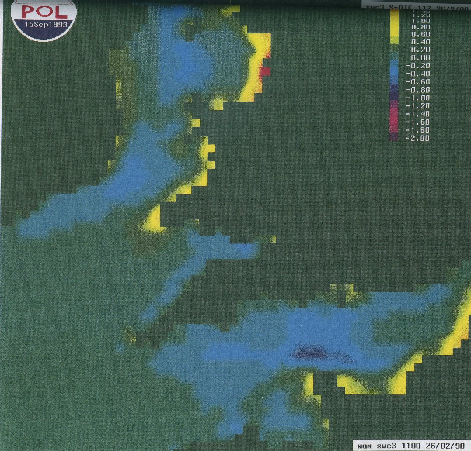
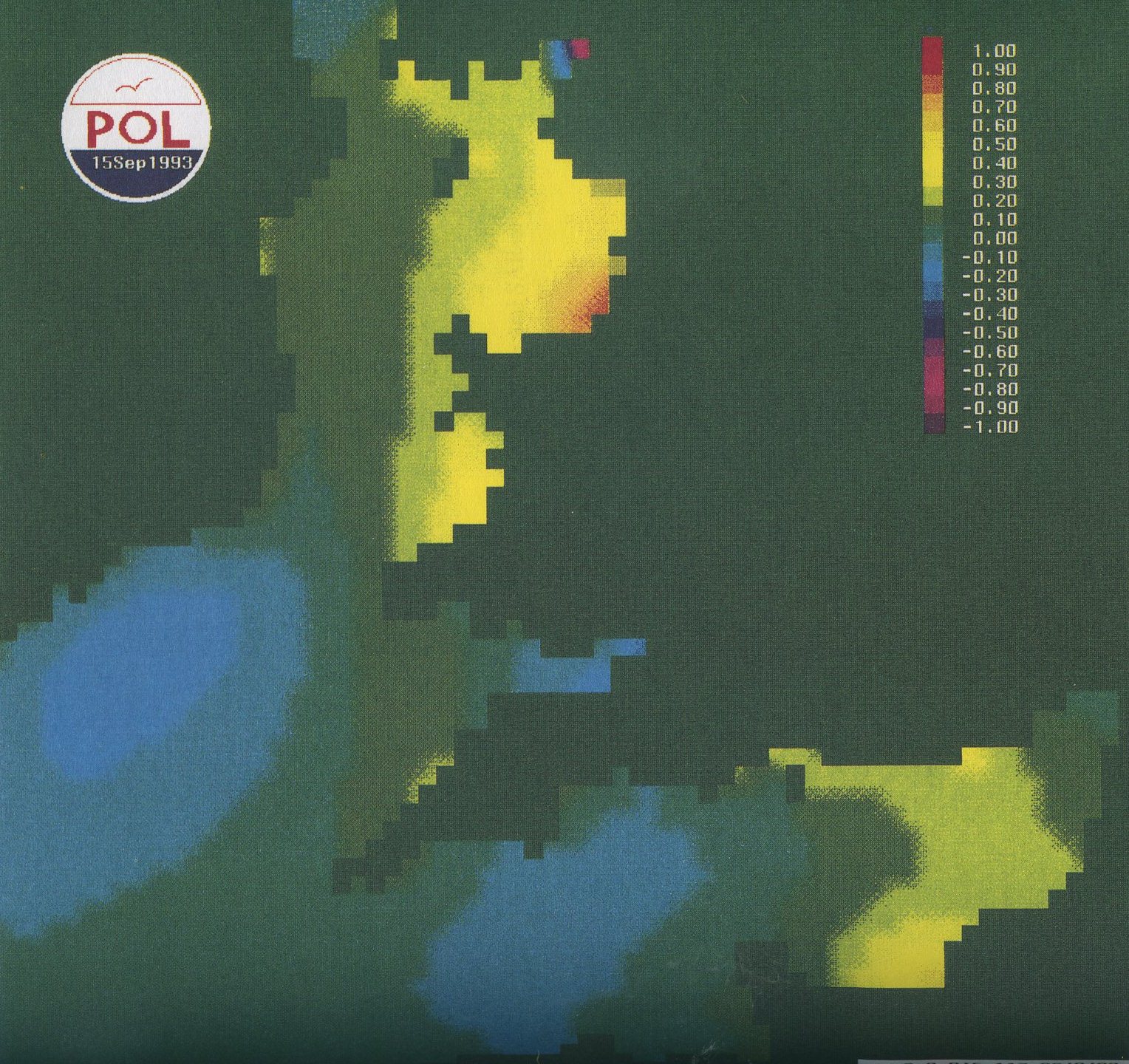
K. P. Hubbert, and J. Wolf Numerical investigation of depth and current refraction of waves. J.Geophysical Research, 96, 2737-2748. (1991)
Wu, X. and R. A. Flather Hindcasting waves using a coupled wave-tide-surge model. pp150-170 in, The Third International Workshop on Wave Hindcasting and Forecasting, Montreal, May 19-22,1992. Preprints, Ontario: Environment Canada, 400pp.
R. M. Thorne, and R. B. Horne The contribution of ion-cyclotron waves to electron heating and SAR-arc excitation near the storm-time plasmapause Geophys. Res. Lett. 19 (1992) 417-420.
Y. Mei, R. M. Thorne, and R. B. Home Ion-cyclotron waves at Jupiter: possibility of detection by ULYSSES Geophys. Res. Lett. 19, (1992) 629-632.
R. M. Thorne, and R. B. Horne Cyclotron absorption of ion-cyclotron waves at the bi-ion frequency Geophys. Res. Lett. 20, (1993) 317-320.
R. B. Home, and R. M. Thorne On the pref erred source location for the convective amplification of ion cyclotron waves J. Geophys. Res. 98, (1993) 9233-9247.
R. B. Home, and R. M. Thorne Oxygen heating via absorption of ion cyclotron waves at the cyclotron harmonic and bi-ion resonance frequencies Proceedings of the ST ART conference, ESA, Aussois, (1993) in press.
Millward, Quegan, Moffett: Upper Atmosphere Modelling Group, School of Mathematics and Statistics, University of Sheffield
Fuller-Rowell: CIRES, University of Colorado/ NOAA, Space Environment Laboratory, 325 Broadway, Boulder, Colorado
Rees: Atmospheric Physics Laboratory, University College London
The global coupled ionosphere/thermosphere/plasmasphere model has been developed by collaboration between the University of Sheffield, University College London and the Space Environment Laboratory, Boulder, and employs large scale numerical finite difference techniques. For a given (and possibly time-dependent) convection electric field, the model calculates the time-dependent global three dimensional structure of the temperature, density, composition and vector velocity of the neutral atmosphere and the density, composition and vector velocity of the ions O+ and H+, by solving the non-linear equations of continuity, momentum and energy. The concentrations of the molecular ion species O+ 2 and NO+ are calculated using a simpler solution scheme which assumes chemical equilibrium, and the electron concentration at each point is then taken to be the sum of the concentrations of the individual ionic species O+, H+, NO+ and O+ 2 (assuming charge neutrality). The solution is performed numerically on a global grid with resolutions of 2 degrees in latitude and 18 degrees in longitude. Each grid point rotates with the earth to define a non-inertial frame of reference in a spherical polar coordinate system, each longitude sweeping through all local times during a 24 hour simulation. In the vertical dimension, the thermospheric code uses 15 grid points corresponding to levels of constant pressure. The pressure levels are separated by a distance equivalent to one scale height, the bottom level forming a boundary defined to have a pressure of 1 Pascal at an altitude of 80 km. The top boundary (pressure level 15) lies at an altitude of between 450 and 600 km, dependent (mainly) on solar activity. In contrast, the ionospheric part of the code (at high latitudes) is divided vertically into 90 fixed heights covering the altitudes 120 to 10,000 km, with coupling in the direction aligned with the earth's magnetic field. A mid-latitude and low-latitude ionosphere/plasmasphere model has recently been developed as an enhancement to the coupled model, and is described in section 3.
This report details recent work which has been conducted using the RAL Cray computers and is presented in two sections. Firstly, a description of recent research into the atmospheric response to transient bursts in the high-latitude convection electric field is given. Secondly, recent coupled model development work and results are described (i.e., the development of a mid and low-latitude ionosphere/plasmasphere model).
The high-latitude ionosphere and thermosphere is a complex region with a structure, to a large degree, dominated by the influence of an electric field, of magnetospheric origin, which controls the motion of the ions and, indirectly, the neutral gas, due to collisions. Recent ground based and satellite studies have indicated that, far from forming a steady state convection pattern, the electric field at high latitudes shows bursts of activity, the bursts repeating over time scales of less than an hour. Such dynamic fluctuations are thought to occur during intervals when the amount of energy input to the magnetosphere from the solar wind is large and there is evidence of an association with a southward turning of the IMF and magnetic reconnection in the magnetotail.
The modelling studies outlined here are motivated by recent high-resolution measurements which show that nightside auroral plasma convection commonly proceeds as a series of periodic, recurrent bursts (see, for example, Figure 1 in Williams et al., 1992). The subject here is the form of the equatorward propagating gravity waves generated by such recurrent events and, in particular, the behaviour due to the periodicity of the electric field bursts. The work builds on previous studies [Millward et al., 1993a; 1993b]. These studies were concerned with the generation and propagation of large scale AGWs resulting from a single short-lived enhancement in the magnitude of the global convection field. Figure 1 shows the generation of a large scale atmospheric gravity wave within the model due to a transient burst of enhanced ion convection in the dawnside high-latitude atmosphere.
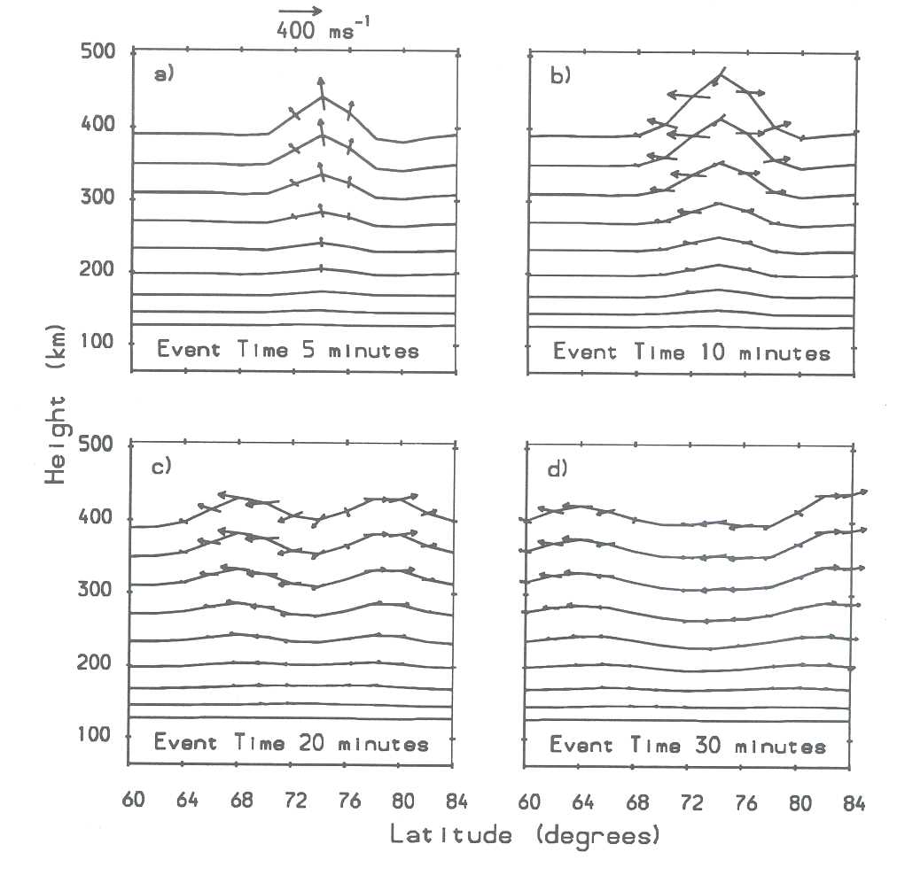
The new work has been concerned with the atmospheric response to a series of consecutive ion bursts and particularly with effects due to the periodicity of the electric field. The individual bursts are of a magnitude smaller than those modelled previously, a factor 0.5 of those used in Millward et al.(1993a), resulting in 'quiet-time' values at the centre of the electrojet region of magnitude approximately 33mVm-1. This increases three-fold at the peak of each burst producing a maximum field of approximately 100mVm-1. (The electric field model used is from the Rice University magnetospheric model [Wolf et al., 1991].)
In five separate experiments, repeated bursts in the electric field are separated by times of 20, 30, 40, 50 and 60 minutes, respectively. A sixth run used a steady-state electric field to produce quiet-time results. Examples of the form of the boost to the electric field are shown in Figure 2.
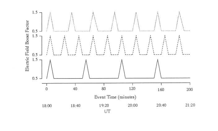
The model was run for December solstice, solar maximum conditions of F10.7 = 185 and a simulation time of 200 minutes, from 18:00 UT to 21:20 UT. Output was made of atmospheric parameters at a typical dawn sector longitude of 162°E. The F-region thermospheric response for electric field periodicities of 20, 30, 40 and 50 minutes is shown in Figures 3a, 3b, 4a and 4b respectively. In all plots, the change in the height of pressure level 12 (at an altitude of roughly 300km), relative to a quiet time run, is plotted as a function of geographic latitude and event time. In Figures 3b, 4a and 4b it can be seen that each burst in the electric field creates a single dominant AGW pulse which propagates equatorwards to mid-latitudes.
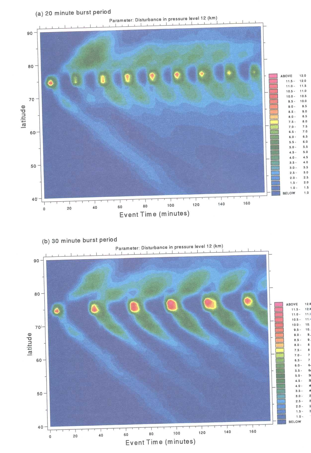
It is clear that, at mid-latitudes, the amplitude of all AGW pulses (after the initial pulse) is larger for the 50 and 40 minute burst periods ( 4a and 4b) than the 30 minute period (3b ). All are larger than the response to a 20 minute period (3a) in which gravity waves are very muted and do not propagate to mid-latitudes. These results are demonstrated further in Figure 5 which plots the disturbance in the height of pressure level 12 at latitude 56°N, relative to a quiet time run, for the five separate experiments. In all cases (except panel a) it can be seen that the periodic electric field produces a gravity wave response at mid-latitudes which has the appearance of a continuous wave with the same periodicity as the driving electric field. It is also seen that the largest amplitude waves are produced for an electric field period of between 40 and 50 minutes (panels c and d). A similar result is obtained at all locations south of, and including, the source region. This is demonstrated in Figure 6 in which the wave amplitude ( excluding the initial pulse) is plotted as a function of the source electric field period for latitudes 74° ( the source region), 66°, 56°, and 40°N.
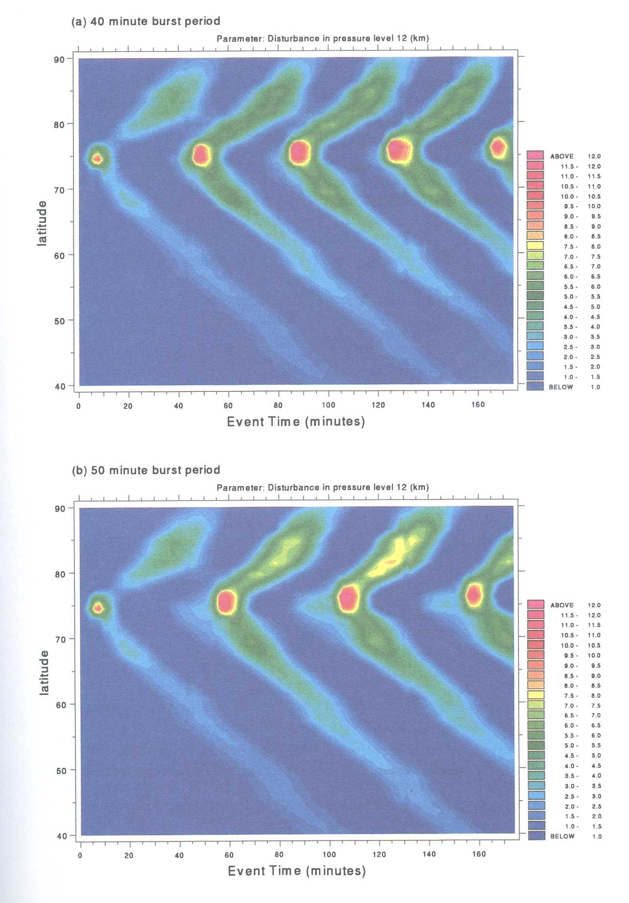
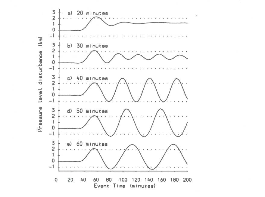
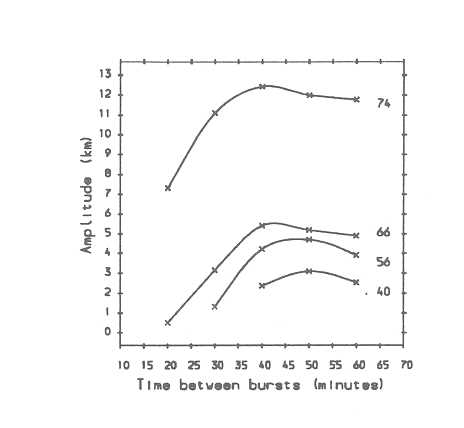
In Millward et al. (1993b) it was shown that the atmospheric response to a single transient burst in the electric field is a heavily damped wave consisting of a dominant initial oscillation, followed by a much smaller, though significant, second oscillation. This result is critical to the present study. The motion of the atmosphere within the source region can be seen in Figure 7 where the change in the height of pressure level 12, relative to quiet time, for the five experiments, is plotted against event time at a source region latitude of 74°N. It can be seen that for electric field periodicities of around 40 and 50 minutes (panels c and d), consecutive bursts in the electric field occur (roughly) in phase with the natural atmospheric oscillation resulting from a previous burst and therefore lead to an enhanced, resonant, response. For shorter electric field periodicities, bursts occur too early to be in phase with the natural atmospheric motion and the amplitude of the AGWs produced is thus more muted. This effect is extremely marked for the case in which the electric field has a periodicity of 20 minutes (panel a). For periods of longer than 50 minutes, successive bursts are also out of phase with the natural oscillation of the atmosphere and lead to smaller amplitude AGWs, although the effect is not so severe.
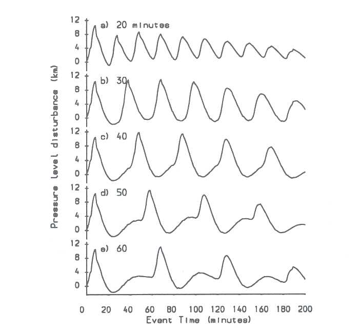
This work is of significance to studies involving the correlation of dynamic high-latitude electric fields and mid-latitude AGW data, such as in the 'WAGS' studies [Williams et al., 1993). Clearly, for an electric field which shows an impulsive nature with periodicities of between 20 and 60 minutes, significant gravity wave responses will occur preferentially for electric field periodicities of around 45 minutes, although this figure will be dependent upon the actual atmospheric conditions, such as the local thermospheric temperature. This selection effect has been confirmed by recent simulations in which a series of electric field bursts, identical to those described here, but spaced 'randomly' in time, have been applied to the model. (This work has recently been accepted for publication [Millward {1994)].)
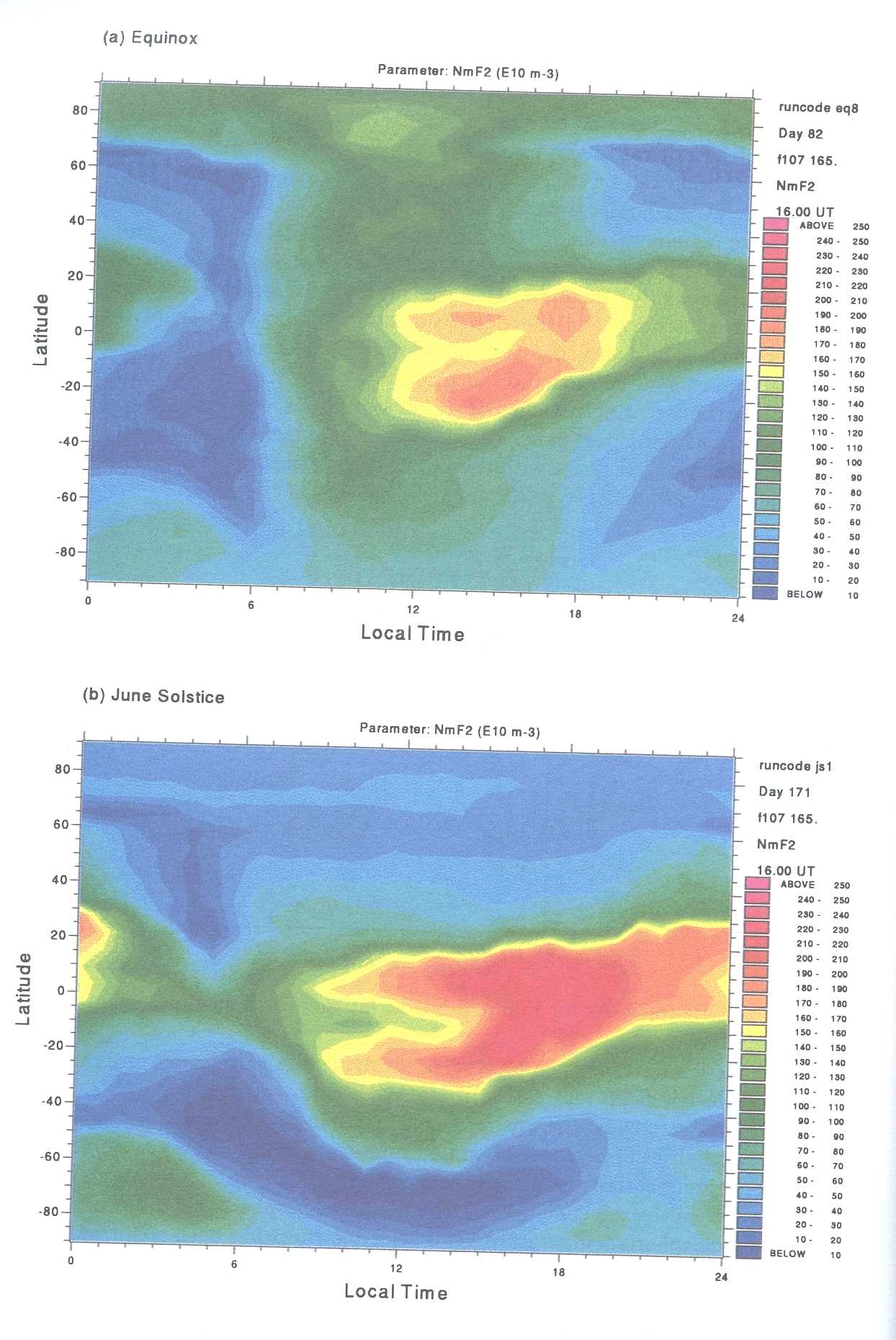
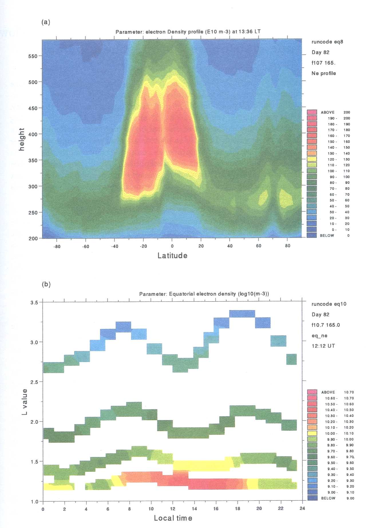
The computational model of the Earth's ionosphere and thermosphere has undergone recent development work to include a fully coupled model of the mid- and low-latitude ionosphere and plasmasphere. The new enhancement calculates the density, temperature and field-aligned velocity of ions O+ and H+ along a flux tube coupling northern and southern hemispheres, the orientation having been determined by an eccentric dipole magnetic field. In order to provide a global picture, a large number of flux tubes spaced in latitude and longitude are computed concurrently. The effects of mid- and low-latitude electric fields are incorporated by allowing all flux tubes to move under E × B drift. This recent development work means that, for the first time, the model is capable of simulating the complete, global ionosphere, whereas previously, only the high-latitude region had been properly included.
An important test for the new enhanced coupled model was that there should be no observable discontinuity in the F-region ion density between the two ionospheric models at the northern and southern boundaries. The main change which was required in order to achieve this was to ensure that the magnetic field model was consistent across the boundary. This was achieved by converting the coupled model as a whole to use an eccentric dipole magnetic field model. Global plots of NmF2 for solar maximum conditions are shown in Figures 8a and 8b for equinox and June solstice respectively. Both plots give 'snapshots' at a universal time of 16:00 UT.
Daytime electron density is shown as a function of height and latitude in Figure 9a for equinox and under solar maximum conditions (F10.7 = 165). The figure shows clearly the global height structure of daytime electron density. At equatorial latitudes, the F2 peak is located at heights of between 350 and 400 km, in contrast to the situation at mid and high-latitudes where the daytime F2 peak is seen to fall between 250 and 300 km. The equatorial anomaly, in which there is a density minimum at the magnetic equator and maxima to the north and south is clear.
In addition to global ionosphere/thermosphere calculations, the new enhanced model also includes a global description of the earth's plasmasphere. Figure 9b shows a global snapshot of plasmaspheric equatorial electron density, as a function of L value and local time. Each of the coloured blocks represents the equatorial density from a single flux-tube, with the format of the figure indicating the resolution of the modelled plasmasphere.
This research has been supported by SERC grant no. GR/H 57295 and has been accomplished using the RAL CRAY XMP and YMP computers under accounts cra384 and cra466.
Millward G H, A resonance effect in AGWs created by periodic recurrent bursts in the auroral electric field, Ann. Geophys., 1994 (in press).
Millward G H, S Quegan, R J Moffett, T J Fuller-Rowell and D Rees, A modelling study of the coupled ionospheric and thermospheric response to an enhanced highlatitude electric field event, Planet. Space Sci., 41, 45, 1993a.
Millward G H, R J Moffett, S Quegan and T J Fuller-Rowell, Effects of an atmospheric gravity wave on the mid-latitude ionospheric F-layer, J. Geophys. Res., 1993b (in press).
Quegan S, G H Millward and T J Fuller-Rowell, A study of the evolution of a highlatitude trough using a coupled ionosphere/thermosphere model, Adv. Space Res. 12, 161, 1992.
Williams P J S, R V Lewis, M Lester, I W McCrea, G H Millward and S Quegan, Correlation of the auroral electric field at EISCAT and travelling ionospheric disturbances over the UK, Adv. Space Res., 1994 (in press)
Williams P J S, R V Lewis, T S Virdi, M Lester, and E Nielsen, Plasma flow bursts in the auroral electrojets, Ann. Geophys., 10, 835, 1992.
Williams P J S, T S Virdi, R V Lewis, M Lester, A S Rodger and K S C Freeman, Worldwide atmospheric gravity-wave study in the European sector 1985-1990, J. Atmos. Terr. Phys., 55, 683, 1993.
Wolf R A, R W Spiro and F J Rich, Extension of convection modelling into the high-latitude ionosphere - some theoretical difficulties, J. Atmos. Terr. Phys., 53,
Computational electromagnetics has been identified as a key technology for enabling the design of advanced aerospace vehicles. The development of suitable computational tools in this area is essential if stringent design requirements, such as low observability, are to be met. In recent years, the time domain method of solution of Maxwell's equations has been developed as an alternative to the more traditional method of moments approach for such problems. This interest in the time domain approach has been driven by the expectation that it should permit the modelling of large problems of current industrial interest, due to its reduced computational requirements[1].
Maxwell's equations, governing the propagation of electromagnetic waves in free space, are considered in the form
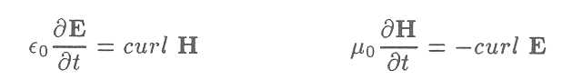
Here E = (Ex,Ey,Ez) and H = (Hx,Hy,Hz) denote the electric and the magnetic field intensity vectors respectively. The dielectric permittivity and magnetic permeability of free space are represented by ε0 andμ0 respectively. Unstructured grid based finite element methods have been the subject of much recent research activity in the area of computational aerodynamics[2]. The major attraction of the unstructured grid approach is its geometrical flexibility and the availability of automatic unstructured mesh generators, which can handle routinely computational domains of arbitrary complex shape. These benefits of the unstructured approach will be of equal importance in the area of computational electromagnetics but they can only be accessed if unstructured grid solution algorithms are developed for Maxwell's equations. For the development of such a solution algorithm, it is convenient to observe that this pair of equations (1) may be expressed alternatively in the conservation form
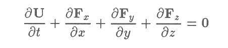
relative to a cartesian coordinate system Oxyz, where
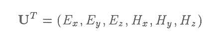
and where the entries in the flux vectors Fx, Fy and Fz are appropriately interpreted. The advantage of working with the equations expressed in this conservation form is that numerical techniques which have already been well developed for the solution of the equations of compressible flow can now be applied here with minor modification.
An advancing front mesh generation method [2] is employed to produce a discretisation of the computational domain into an unstructured assembly of linear 3-noded triangular elements. The algorithm which has been adopted to advance the solution for the scattered field in time on such meshes is an explicit two-step finite element based Taylor-Galerkin procedure [3], which is notionally second order accurate in both time and space.
The research to date has concentrated upon problems involving the scattering of electromagnetic waves by perfectly conducting obstacles. For single frequency incident waves of the form
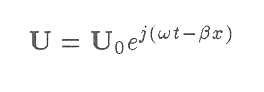
where U0 is a constant and j = √(-1), the solution is advanced in time through a prescribed number of cycles until 'steady' conditions are achieved. A further cycle is then computed, during which time the solution at each vertex in the mesh is monitored to determine the amplitudes and the phases of the components of the scattered electric and magnetic fields. Far field scattering data can be obtained from the results of the the time domain computation by employing a near-field to far-field transformation.
The computational approach has been validated by comparing computed and exact solutions for problems involving the scattering of plane TE and TM waves by an infinite circular cylinder. The method is currently being applied to scattering problems involving shapes of industrial interest, such as aerofoil sections and cavities. The computed magnetic field for a problem involving the scattering of a TE wave by a cavity is shown in Figure 1.
The computations reported here were performed interactively on the SERC CRAY YMP at the Rutherford Appleton Laboratory using computer time provided under Grant GR/G 59240. Colouring of the elements in the mesh ensures that the computer code can be fully vectorised and a highly efficient computational procedure results. The typical memory requirements are around 1.5 Mwords for a mesh of 50,000 triangular elements and run times of the order of 10 minutes are required to perform 800 time steps.
Support for this work is also provided by the Department of Computational Engineering, Sowerby Research Centre, British Aerospace plc.
1. A. Taflove, 'Re-inventing electromagnetics: supercomputing solution of Maxwell's equations via direct time integration on space grids', AIAA Paper 92-0333, 1992
2. K. Morgan, J. Peraire and J. Peiro, 'Unstructured grid methods for compressible flows', in AGARD Report R-787: Unstructured Grid Methods for Advection Dominated Flows', AGARD, Paris, 5.1-5.39, 1992 3.
K. Morgan, J. Peraire, J. Peiro and 0. Hassan, 'The computation of three dimensional flows using unstructured grids', Comp. Meth. Appl. Mech. Engng. 87, 335-352, 1991
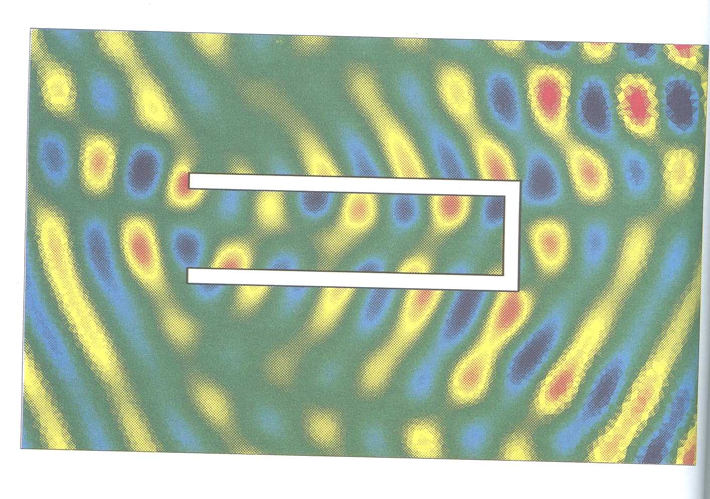
The Cray Computers have been used under a 'facilities-only' grant to enable large-scale computations of electromagnetic field distributions to be undertaken in support of a variety of projects, as outlined in separate sub-sections below.
A method for generation of a close approximation to an electromagnetic plane wave, using an array of antennas, is being developed at Bradford. Computer modelling of this involves computation of the field generated in the test zone due to each antenna element in turn, synthesis of the optimum phase and amplitude relationship between the elements using a least-squares technique, and ultimately computation of the resulting field in the test zone when all array elements are excited together in the approximate relationship. An integral-equation technique is used for the first and third stages, the industry-standard numerical electromagnetics code (NEC) being the chosen software. This involves the solution of a large set of linear equations, a task well-suited to a vector processor. A typical result for the field distribution in the test zone is shown in Fig 1; this demonstrates good uniformity over the central region, as required.
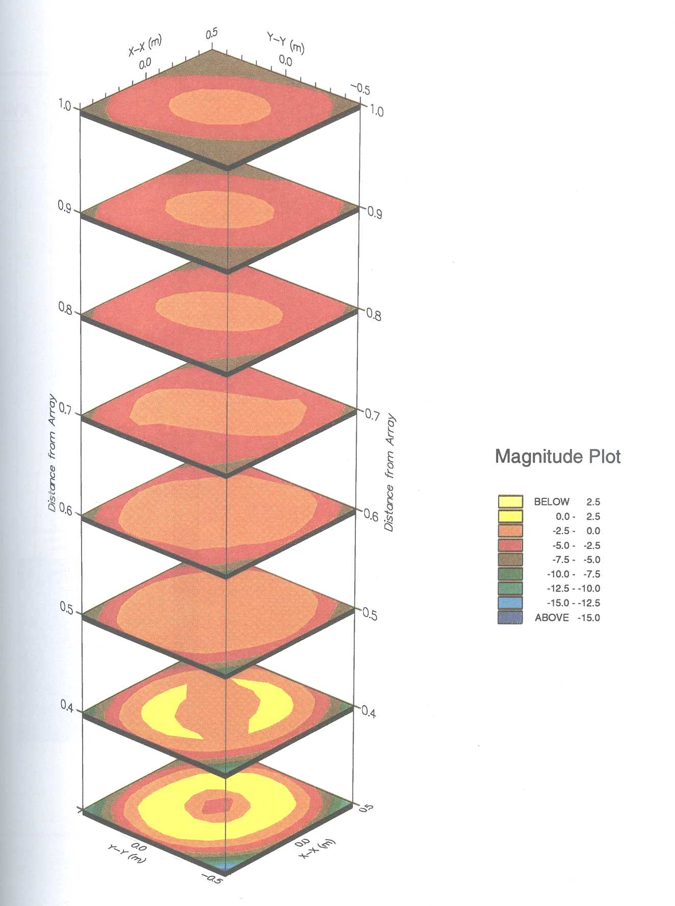
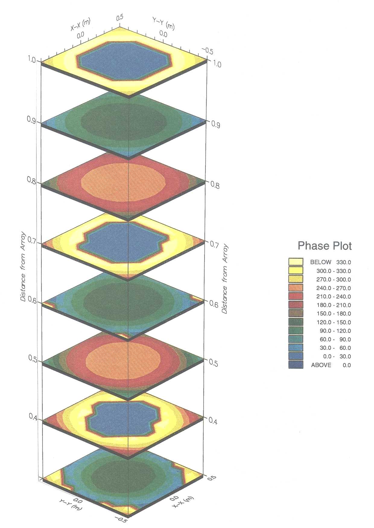
In a separate exercise, the NEC was restructured in order to maximise its running speed on the Cray X-MP. Four techniques were used for different parts of the program: vectorisation, autotasking, microtasking and macrotasking. The initial speed with automatic vectorisation switched on was 20 MFlops. Using hand vectorisation this was increased to 68 MFlops.
When autotasking was invoked to exploit the parallelism of the machine ( 4processors on the X-MP), no significant increase in speed was found. However, with careful hand application of microtasking and macrotasking to different parts of the code, an increase to a speed of the order of 100 MFlops ( depending on the nature of the problem being addressed) was achieved, a reasonably good speed for a 'real application' code on this machine. It was concluded that optimum exploitation of a vector-parallel machine requires an intimate understanding of the total task, including the physics of the problem, the mathematical formulation, the design of the algorithm, and the architecture of the computer. All of these components are strongly interdependent, and the machine architecture can thus influence very fundamental decisions on the choice of approach to be used. For instance, a distributed-memory parallel processor would favour the differential-equation approach to field computation, whereas the integral-equation approach tends to run more efficiently on a shared-memory machine.
For this work a finite-difference frequency-domain program was used, requiring the computation of the field over a dense matrix of points within the cavity dielectric. The object was to discover the modes that would exist within a cavity, their resonant frequencies, and the way in which they interact with the walls. The effect of loading with dielectric-resonator material was also investigated; an example of a typical field distribution is shown in Fig 2.
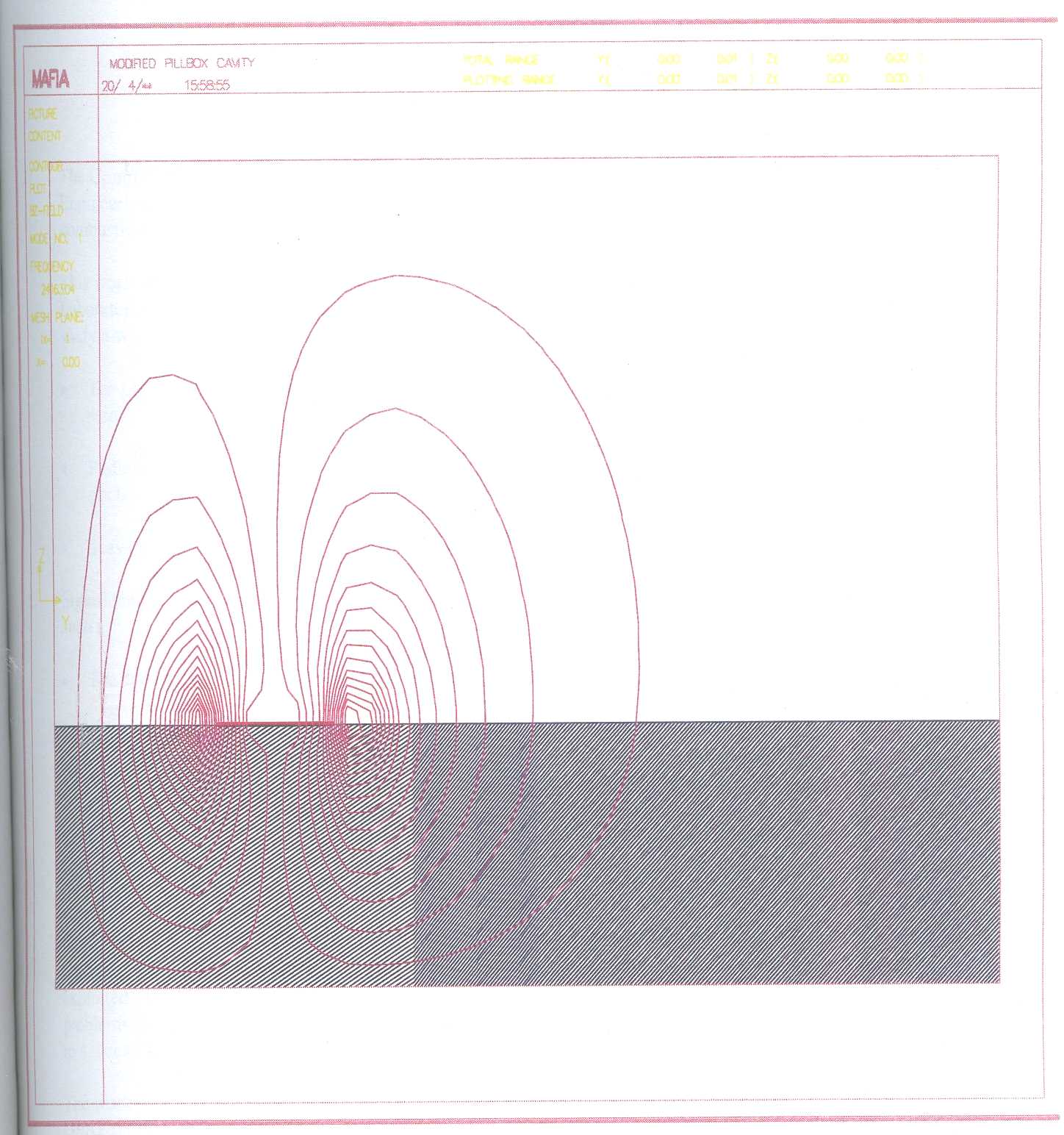
In a related project, the Cray Y-MP has also. been used to model a helical antenna that has been identified as a propitious design for realisation in superconductor. This has been modelled using a new integral-equation technique, generating a task similar in size to that for the electromagnetic test facility (above).
A finite-difference-time-domain program is being used to calculate radio frequency field distributions in the human head, in order to ensure compliance of radio systems with safety standards limiting the peak acceptable field strength. The grid of data points involved (up to 10 million) is far larger than can be handled by ordinary computers, since a very fine-resolution simulation of the head is required so that possible fine-structure effects are not overlooked. (This work is still in its early stages).
P S Excell, N N Jackson, & K T Wong A Compact Electromagnetic Test Range using an Array of Log-Periodic Antennas IEE Proceedings Part H 140 (1993) 101-106
P S Excell Computational Electromagnetics in Education at the University of Bradford, England IEEE Trans. Education 36 (1993) 227-229
A E Centeno, & P S Excell High Q Dielectrically Loaded Electrically Small Cavity Resonators IEEE Microwave and Guided Wave Letters 3 (1993) 173-4
P S Excell, & K W Yip Optimisation of the Numerical Electromagnetics Code on a Four-Processor Cray XMP Computer IEE Conf. Pub. No. 350 'Computation in Electromagnetics', London 1991, 55-58
PS Excell, & N N Jackson Compact Range Illumination using an Array of Log-Periodic Dipole Antennas IEE Conf. on Electromagnetic Compatibility, Edinburgh, 1992, 181-188
PS Excell, & N N Jackson UHF Compact Range Illumination using an Array Antenna DTI/SERC Joint Framework for Information Technology Technical Conference Digest, Keele 1993, 275-282
N N Jackson, & P S Excell An Active Array for a UHF Compact Range IEE Conf. Pub. No 370 'Antennas & Propagation', Edinburgh 1993, 388-391
R A Abd-Alhameed, & P S Excell Computer Modelling of Superconducting Helical Antennas IEE Conf. Pub. No 370 'Antennas & Propagation', Edinburgh 1993, 496-499 _
N N Jackson, & P S Excell A Compact Range Using an Array Antenna IEE Colloquium Digest No. 1992/132 'Radiated Emission Test Facilities', London 1992 3/1-3/5
P S Excell, G J Porter, Y K Tang, & K W Yip Re-working of Two Standard Moment-Method Codes for Execution on Parallel Processors IEEE Conf. on Electromagnetic Field Computation, Los Angeles 1992, paper TP40
A Centeno, & P S Excell Computer Aided Design of Dielectric Filter Elements using a Rigorous Numerical Technique IEE Colloquium Digest 1992/220, 'Filters in RF and Microwave Radio Communications', Bradford 1992, 8/1-8/4
The Computational Fluid Dynamics (CFD) Modelling Group in the Department of Mechanical Engineering at Loughborough University of Technology, has been involved primarily with engine combustion and associated pollutant formation and heat transfer problems since 1989.
This work has been undertaken with the CFD code KIV A-II, developed at the Los Alamos Laboratories in the US. The code has been extended considerably by the Loughborough Group to study a wider range of problems than addressed with the original code, these are:
Significant changes to the original code were necessary in its application to free boundary problems such as:
In all this work the availability of the Cray computing resources at Rutherford have been invaluable, particularly in regard to the free boundary problems above which in the main involved large three dimensional domains.
The computing facilities at Loughborough consist of networked HP750 processors which are adequate for code development and small to medium sized tasks where system symmetry can be exploited. However, once code has been developed, parametric studies using the code present problems in regard to data storage. The free boundary problems discussed above can take between 2 to 4 weeks to run on a single HP750 which is acceptable during model development and research.
The work outlined here has been supported through the following SERC grants GR/F2178.7, GR/G25177 and GR/H82136.
The availability of the high speed (Super-JIPS) link between Loughborough and Rutherford will enhance our usage of the Cray services. However, this will also result in faster consumption of allocated computational resources. There needs to be a more flexible and streamlined procedure for topping up computational resources in the course of a project. It is not always possible to accurately assess computational resources at the outset of a project and investigators are usually reluctant to build in large factors of safety into their estimates.
Separated flow regions, even if small, can have profound consequences to the overall behaviour of the flow containing these regions, and thus to the performance characteristics of the associated fluid-engineering device. The loss of lift of an aerofoil at high incidence due to suction-side separation, and of pressure recovery in a stalled turbomachine passage are two especially important, closely related examples.
Modelling separation and recirculation accurately is a challenging task, particularly if as is the case in the aforementioned instances - separation occurs at a gently curving surface. One key ingredient to success is a faithful representation of the structure of the curved and decelerating near-wall boundary layer approaching the separation line, for this will have a considerable effect on the location of separation and hence on the ensuing recirculation pattern.
Once separation has occurred, the flow becomes highly curved, turbulence transport is anisotropic and the reattachment behaviour is strongly influenced by the wall and the turbulence structure in the curved shear layer emanating from the separation line. Although the structure within the recirculation zone is rarely of primary interest, it strongly affects the overall shape of the recirculation zone, the point of reattachment and the recovery behaviour of the wake following reattachment. Hence, the details within the recirculation zone need also to be resolved accurately.
The recognition of the prominent role played by flow curvature and turbulence anisotropy in damping or augmenting turbulence transport has given strong impetus to studies investigating the predictive capabilities of a class of turbulence models which solve transport equations for statistical correlations of turbulent velocity fluctuations - a framework termed "second-moment closure". The overwhelming majority of the studies undertaken so far have focused on two-dimensional separation from sharp edges or induced by strong swirl or shocks. The study reported here aims to contribute to a clarification of the capabilities of different forms of second-moment closure in predicting separation specifically from curved surfaces. Calculations are presented for two well-documented laboratory flows:
In the latter case, transition to turbulence is forced at a distance of 0.2 times the body's axis, and leaward separation is of the open type. In the former case, the location of transition is free, but known to have occurred at 0.12 of chord.
The availability of Cray Y-MP resources, particularly the large memory it offers, was crucial in obtaining results for the three-dimensional body with sufficiently fine grid.
Two forms of Reynolds-stress model feature in computations to be presented later, in addition to an eddy-viscosity model which assumes directional isotropy of the turbulence exchange process. Both models solve (for 3D conditions) 6 transport equations for the independent auto- and cross-correlations of turbulent velocity fluctuations, but differ in terms of one particular model fragment responsible for steering turbulence towards isotropy in the absence of fluid straining and shearing (Lien & Leschziner [1,2].
Neither form of the above second-moment closures is applicable for low Reynolds number regions in which fluid viscosity interacts with turbulence. The low turbulence layer very close to wall is one such region, and this needs to be resolved by a special "near-wall model". In the calculations to follow, two alternative near-wall eddy-viscosity variants have been used, one involving the solution of a transport equation for turbulence energy and an algebraic prescription of the turbulence length scale (representing the size of energetic eddies) and the other involving two differential equations, one for turbulence energy and other the rate of dissipation of that energy (Lien & Leschziner [3]).
A general-geometry finite-volume scheme (Lien & Leschziner [1-3]) has been employed to generate the present predictions. This scheme entails a fully collocated storage arrangement for all transported properties, including, if applicable, the Reynolds-stress components. Within the arbitrary (structured) non-orthogonal finite-volume system, the velocity vector is decomposed into its Cartesian components, and these are the components to which the momentum equations relate. As an alternative, the present scheme allows an 'adaptive' decomposition whereby one of the Cartesian components may be adapted to a user-defined datum line. Advective volume-face fluxes are approximated using either the second-order upwind scheme or an upstream weighted quadratic scheme or a so-called "TVD MUSCL" scheme, the last ensuring freedom from spurious oscillations which can arise from dispersive errors associated with high order of interpolation. At all speeds (including supersonic conditions), mass continuity is enforced by solving a pressure-correction equation which, as part of the iterative sequence, steers the pressure towards a state at which all mass residuals in the cells are negligibly small.
Calculations have been made for two principal geometries: a turbulent flow around an aerofoil at 13.3° incidence [4] and a flow around a 1:6 prolate spheroid at 10° incidence. In the former, a "C-grid" containing 356×66 grid nodes was used, extending to 5 chord lengths into the inviscid stream. Experiments show this flow to be separated towards the rear of the upper suction side (i.e., the aerofoil is "stalled").
A partial view of the 170,000-node grid surrounding the prolate spheroid is shown in Fig. 1. Separation is here of the open type, that is, only the azimuthal velocity component reverses its direction in the leaward portion while the streamwise component remains positive. Extensive and very detailed experimental data for velocity, skin friction, direction of surface streak lines and pressure are here available for validation [5].
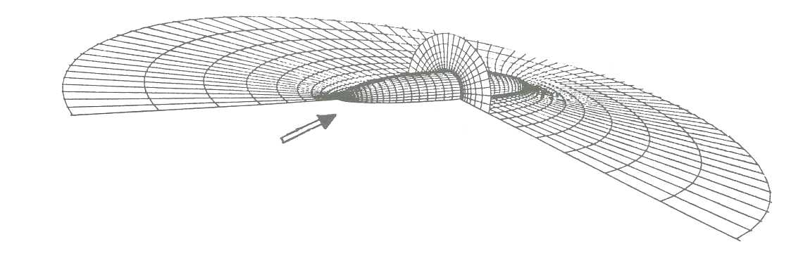
The sensitivity of the pressure distribution around the aerofoil to the turbulence representation is generally weak. This is exemplified by Fig. 2 which contrasts solutions predicted with various models against experimental data . While a relatively modest sensitivity is an expected outcome - for inviscid processes govern the momentum balance - the low level of variability across the entire range of models, particularly at the trailing-edge portion of the suction side, is surprising and indicative of a low sensitivity of the velocity field to turbulence modelling. A somewhat greater variability is displayed by the skin friction, distributions which are given in Fig. 3, and this reflects the importance of modelling accurately the region very close to the wall.
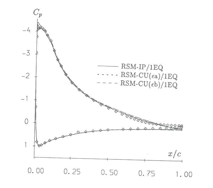
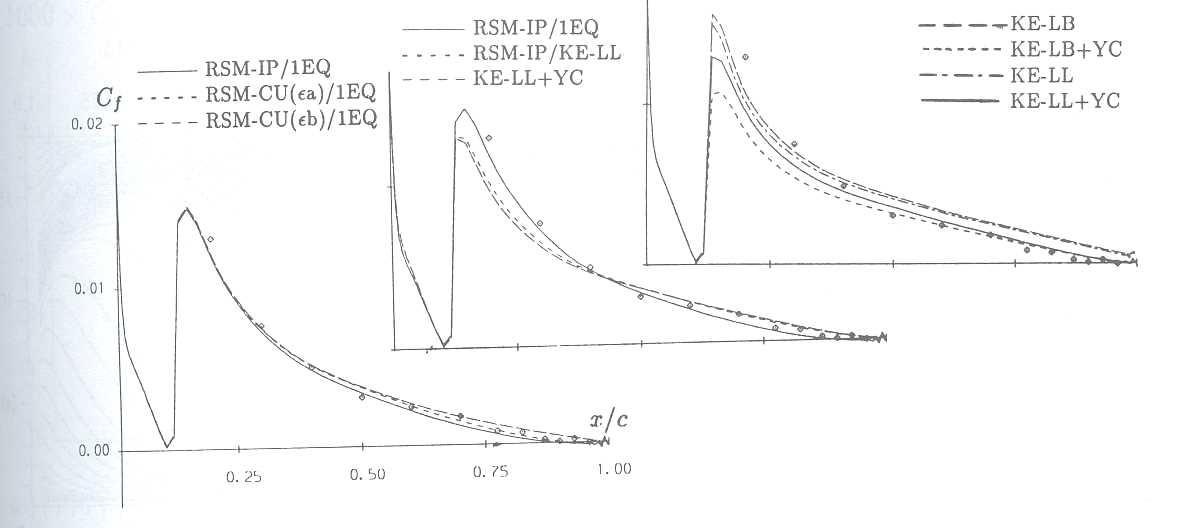
Fig. 4 shows streamwise velocity profiles at 2 stations along the aerofoil's suction side suction. It is noted first that none of the models is able to capture correctly the extent lateral structure of the reverse-flow region. Those models which return negative skin-friction values do so because of a very minor flow reversal along the surface; in contrast, the measurements show a much thicker reverse-flow region and hence much larger displacement. This is clearly a consequence of defects in the turbulence representation in the outer region, away from the wall.
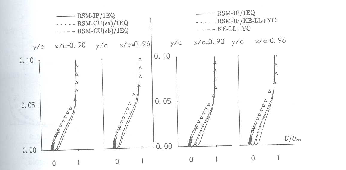
An overall view of the flow around the prolate spheroid is conveyed in Fig. 5 by way of experimental and computational surface streaklines on the spheroid's surface, mapped onto a plane square. The flow progresses from the windward lower left-hand portion to separation at the upper right-hand corner. Both turbulence models, the second-moment one coupled to the near-wall eddy-viscosity form in the near-wall region, return a qualitatively credible representation. Closer examination shows the second-moment closure to predict a more extensive separation zone, however.
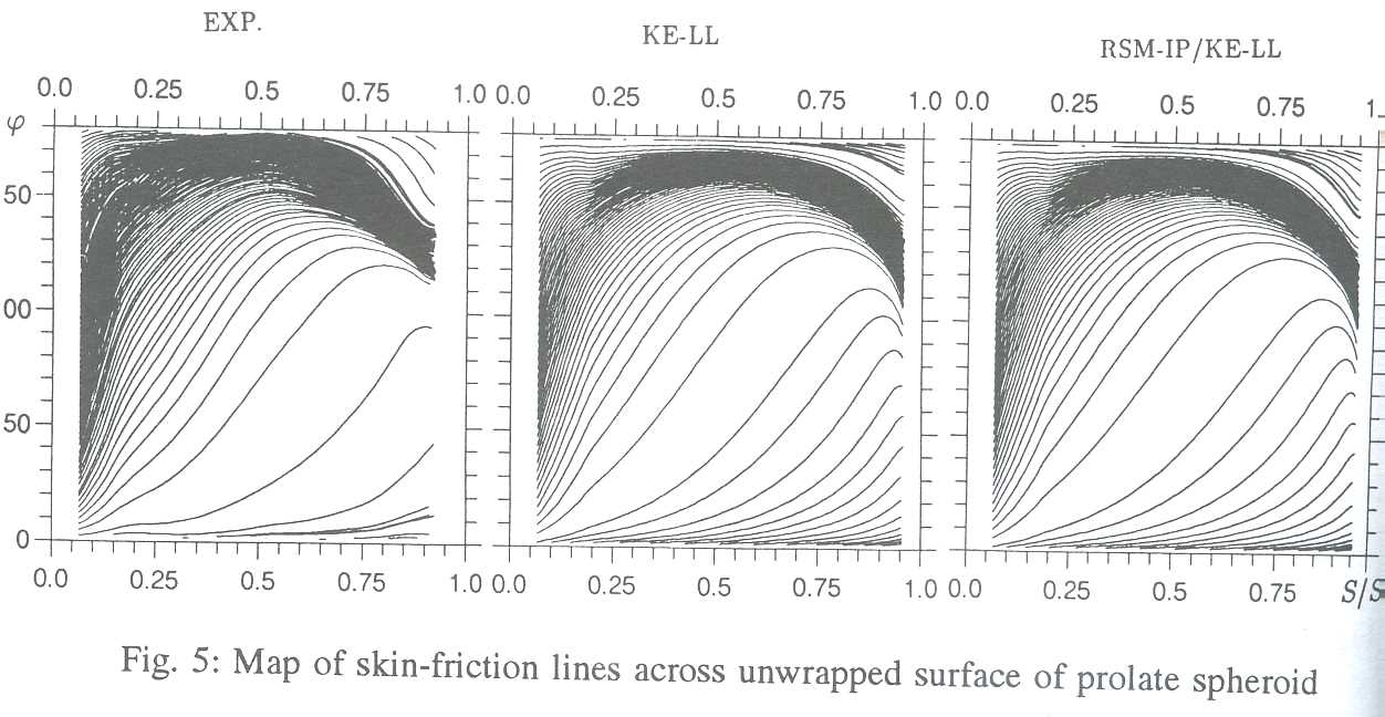
Nose-to-tail pressure distributions at two out 42 azimuthal locations are given in Fig. 6.
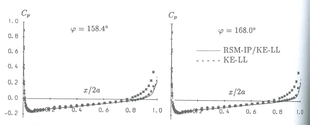
Each contains 4 variations: two computed, one experimental and the fourth arising from the inviscid solution. There is only a small difference between the computed variations, both being fairly close to the experimental data. Worthy of note is the tendency of the second moment closure to capture the inflexion of the experimental variation close to the tail.
Azimuthal variations of total skin-friction at two out of 12 streamwise locations are shown in Fig. 7. Both positions are close to the tail where differences between computations and experiment are largest. These differences are clearly significant: both models underestimate the distortions of the flow associated with flow reversal. However, the second-moment closure returns improved trends, presumably as a result of curvature in the boundary layer attenuating mixing and of stress transport being correctly represented.
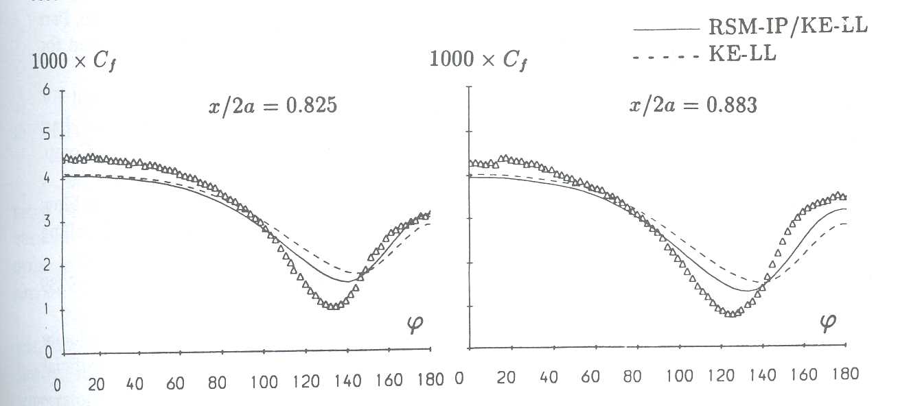
Experimental profiles of stream wise and azimuthal velocity are available at a total of 48 locations across the spheroid's surface. Of these only three are considered in Fig. 8. All locations are at 0.73 of cord - the most rearward position for which data are available - and convey variations in the flow as the separated zone is traversed azimuthally. The azimuthal-velocity profiles provide the clearest evidence of the superiority of the second-moment closure: separation occurs earlier, is more intense and covers a greater lateral distance. Moreover, the distortion of the stream wise velocity profiles, arising from azimuthal convective transport of streamwise momentum, is better captured. Clearly, however, agreement with experiment is not close, and it would appear that the level of shear stress is still excessive - an inference consonant with observations made in the previous aerofoil geometry.
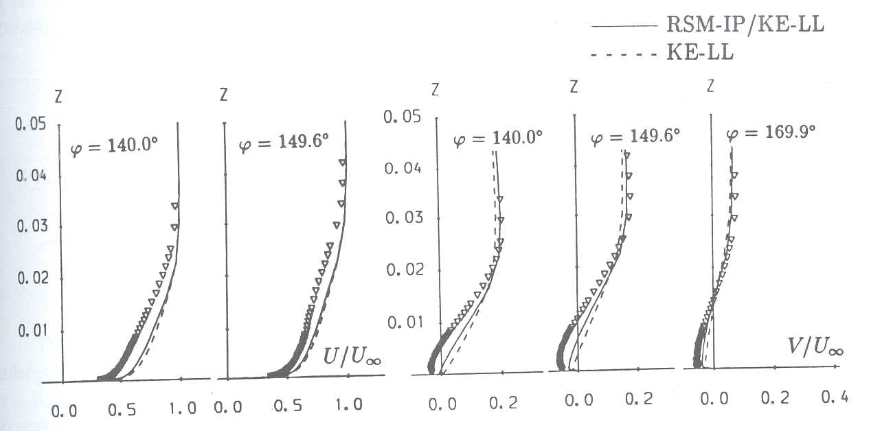
Current efforts focus on investigation of different types of turbulence models and further geometries, both two- and three-dimensional, and the Cray Y-MP continues to play an essential role in this research.
1. Lien, F.S. and Leschziner, M.A., (1992), "A General Non-Orthogonal Collocated FV Algorithm for Turbulent Flow at All Speeds Incorporating Second-Moment Closure, Part 1: Computational Implementation", Technical Report TFD/92/4, UMIST. Accepted for publication by Comp. Meth. Appl. Mech. Engrg. (in press)
2. Lien, F.S. and Leschziner, M.A., (1993), "A General Non-Orthogonal Collocated FV Algorithm for Turbulent Flow at All Speeds Incorporating Second-Moment Closure, Part 2: Application" Technical Report TFD/93/5, UMIST. Accepted for publication by Comp. Meth. Appl. Mech. Engrg. (in press).
3. Lien, F-S and Leschziner, M.A. (1993), "Computational Modelling of 3D Turbulent Flow in S-Diffuser and Transition Ducts", 2nd Int. Sym. on Engineering Turbulence Modelling and Measurements, May 31 - June 2, Florence, Italy.
4 Piccin, 0. and Cassoudesalle D., (1987), "Etude dans la soufflerie Fl des profiles AS239 et AS240", Technical Report P.V. 73/1685 AYG, ONERA.
5. Meier, H.U., Kreplin, H.P., Landhauser, A. and Baumgarten, D., (1984), "Mean velocity distributions in 3D boundary layers developing on a 1 :6 prolate spheroid with artificial transition, DFVLR Report IB 222-84 A 11.
Multiple jet injection followed by impingement on solid surfaces is encountered in a wide range of engineering applications involving cooling, heating, drying, mixing, cleaning and intentional erosion. The process can therefore be said to be generic in nature and of general fluid dynamic interest The particular context of this study is vertical or short take-off and landing of aircraft.
Near-ground operation of such aircraft entails the ejection of two or more high-speed hot jets, followed by ground impingement, the formation of wall jets, the collision of these jets and, finally, the generation of upward-directed fountains (Fig. 1). The intensity, structure and temperature of the upwash are of considerable importance to the operational stability of the aircraft and to the performance characteristics of the engines, the latter associated with the reingestion of the hot and possibly contaminated fountain gases. The interaction between the wall jets and ground-based structures may be an additional factor of interest.
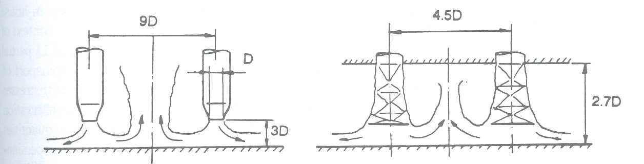
The complexity of the physical processes at play and their intricate interaction pose strong challenges to any modelling strategy, be it based on deterministic or statistical principles. The strain field is highly three-dimensional and turbulent; it is marked, in particular, by severe curvature in the shear layer at the jet and fountain edges close to the primary Get-ground) and secondary (wall-jet) impingement zones, which can have profound consequences to the turbulence level in the shear layers; the impingement process entails severe normal strains which generate turbulence at a rate crucially affected by the level of normal-stress anisotropy, particularly close to the wall; if the jet is under-expanded, its structure is affected by shock and expansion waves which may amplify turbulence and invalidate the scaling laws pertaining to their incompressible counterparts. In the context of a statistical treatment, in which the effects of turbulence are represented in a time-averaged sense by a turbulence model, the above processes call for the use of general differential models which are capable of resolving turbulence transport and accounting, additionally, for the experimentally observed subtle interaction between flow curvature, compressive strain and turbulence anisotropy.
From a numerical point of view, the principal challenge is to adequately support widely disperate scales on what is - unavoidably, in a three-dimensional context - a relatively coarse computational mesh. In particular, there is a need to support the relatively thin curved and highly sheared jet and fountain edges and to resolve the structure of shock-related features whose orientation and spatial location are quite different from those associated with shear. The difficulties introduced through the above disparity of scales are further aggravated by the unconfined nature of the flow and the influence of far-field processes on the jet-fountain structure, which demand the extension of the solution domain to regions far removed from the jets. Clearly, these conflicts and constraints demand the use of accurate, numerically "non-diffusive" approximation scheme but these give rise to stability problems which are considerably aggravated by the highly non-linear and coupled nature of the equations constituting the type of turbulence model needed to resolve the aforementioned physical processes.
At UMIST, a wide-ranging programme of research has been underway over the past three years focusing on the prediction of three-dimensional single and multiple jets, with and without crossflow and impingement [1-4], employing a class of turbulence models which solve transport equations for turbulence correlations interpretable as apparent normal and shear stresses (6 in all three-dimensional flows). Although this modelling framework is particularly resource intensive much of this work has been undertaken on low-performance workstations because of memory constraints of supercomputers accessible to the writers. With the introduction of the Cray Y-MP at RAL with its large memory, the opportunity arose to extend the investigation to more challenging flow conditions, in particular in transonic jets, with a reasonable level of confidence in the numerical accuracy achieved by use of fine grids.
The present summary reports some aspects of ongoing computational studies of twin impinging jets without crossflow, undertaken with the aid of the Cray Y-MP in the period February to July 1993.
The calculations reported herein have been performed using a general-geometry in-house finite-volume algorithm for three-dimensional incompressible flow and extended in the context of the present study to compressible conditions. The algorithm solves the coupled system of 11 partial differential equations describing the conservation of mass and momentum and the transport of turbulence correlations for the time-averaged velocities, pressure and Reynolds (turbulent) stresses in an iterative manner with a "pressure-correction approach" used to satisfying mass conservation indirectly through a progressive adjustment the pressure field. Convection of mean-flow quantities is approximated by a bounded variant of the quadratic approximation scheme in which dispersion-induced oscillations due to the high order of the scheme are removed by means of a non-linear damping algorithm which introduced artificial diffusion when detecting local oscillations. Unusually, this approach, suited principally to incompressible conditions, has been retained for transonic flow, but a number of special practices had to be devised to enable shocks to be captured cleanly [4].
Results are reported here for the two flows sketched in Fig. 1, the first being a twin water jet [6] and the second a similar arrangement of under-expanded air jets discharged at nozzle pressure ratios (NPR) ranging between 2.6 and 3.3 [7]. At the upper NPR limit, the Mach number in the jet reaches a maximum value of about 2.5 . For the former, experimental aerodynamic data were obtained with LDA techniques, while for the latter, the data comprises static and dynamic pressure data, supplemented by Schlieren photographs.
For the incompressible case, essentially grid-independent solutions have been obtained with a mesh containing 85,000 nodes. This number of nodes had to be increased to about 400,000 for the transonic case to adequately resolve shock-induced features. As will be demonstrated below, the latter flow is time dependent due to shock-induced oscillations. This required CPU-intensive time-tracking to be undertaken in order to determine the oscillation frequency and the time-averaged solution. In this case, typical resource requirements were 80 Mb of memory and 6-10 CPU hours per run.
Solutions obtained for the incompressible case with two turbulence models are compared with experimental data in Figs 2-4. Both models are observed to predict similar flow structures in the jets approaching the ground, in the impingement zone and in the initial stages of the fountain, although the more advanced Reynolds-stress model returned a somewhat narrower jet, in better accord with experimental data. As is evident from Fig. 3, significant differences arise, however, as the fountain develops. Thus, the k-e model predicts excessively peaky velocity profiles and a correspondingly low fountain width. In contrast, the Reynolds-stress model returns a much improved representation of the fountain, reflecting a greater sensitivity of this model to curvature-turbulence interaction as the wall jets curve and merge into the fountain. The superiority of the stress model is particularly well brought out in the comparison of the fountain half-width given in Fig. 4.
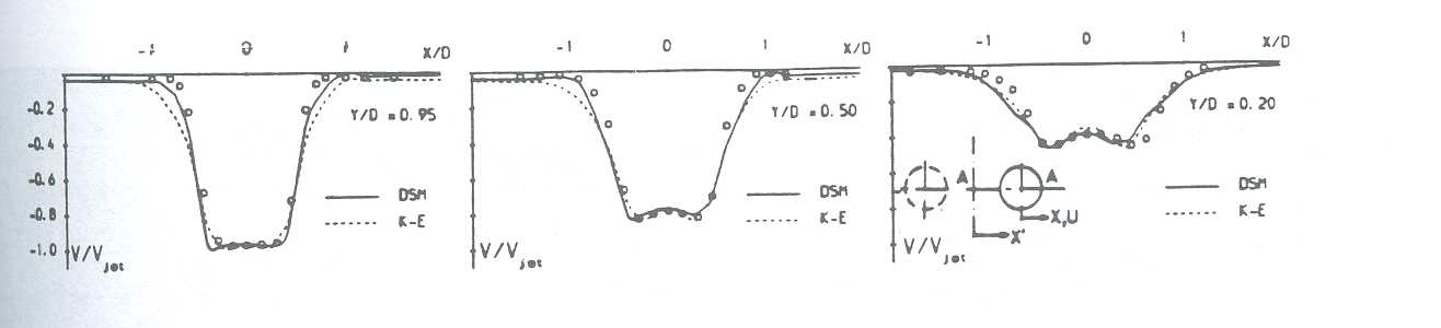
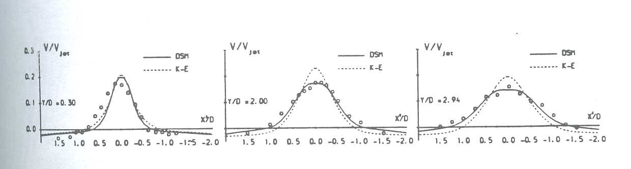
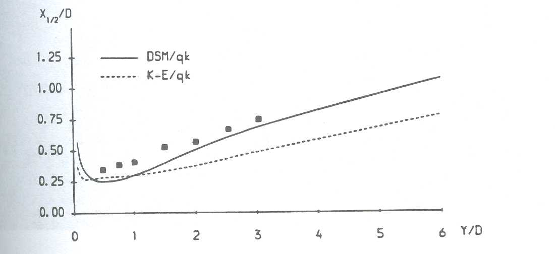
Results for the transonic jets are given in Figs. 5-7. The first gives an overall '3D' view of the impingement process and the fountain predicted at NPR=3.0. Red regions identify high speed flow while blue indicates low velocities. The red patches within the jet signify the existence of 'shock cells' typical of under-expanded jets. A qualitative comparison between predicted and visually observed shock structure is given in Fig. 6. This compares fields of iso-Mach-number contours predicted by the Reynolds-stress model for NPR = 2.6, 3.0 and 3.3 with hand-drawn abstractions obtained from Schlieren photographs which highlight the shock cells and the stand-off shock above the impingement zone. The number and size of the shock-cells observed vary with the NPR value, and this sensitivity is broadly returned by the calculations. Moreover, the stand-off shock is clearly recognizable and has been captured at the experimentally recorded elevation above the impingement plate.
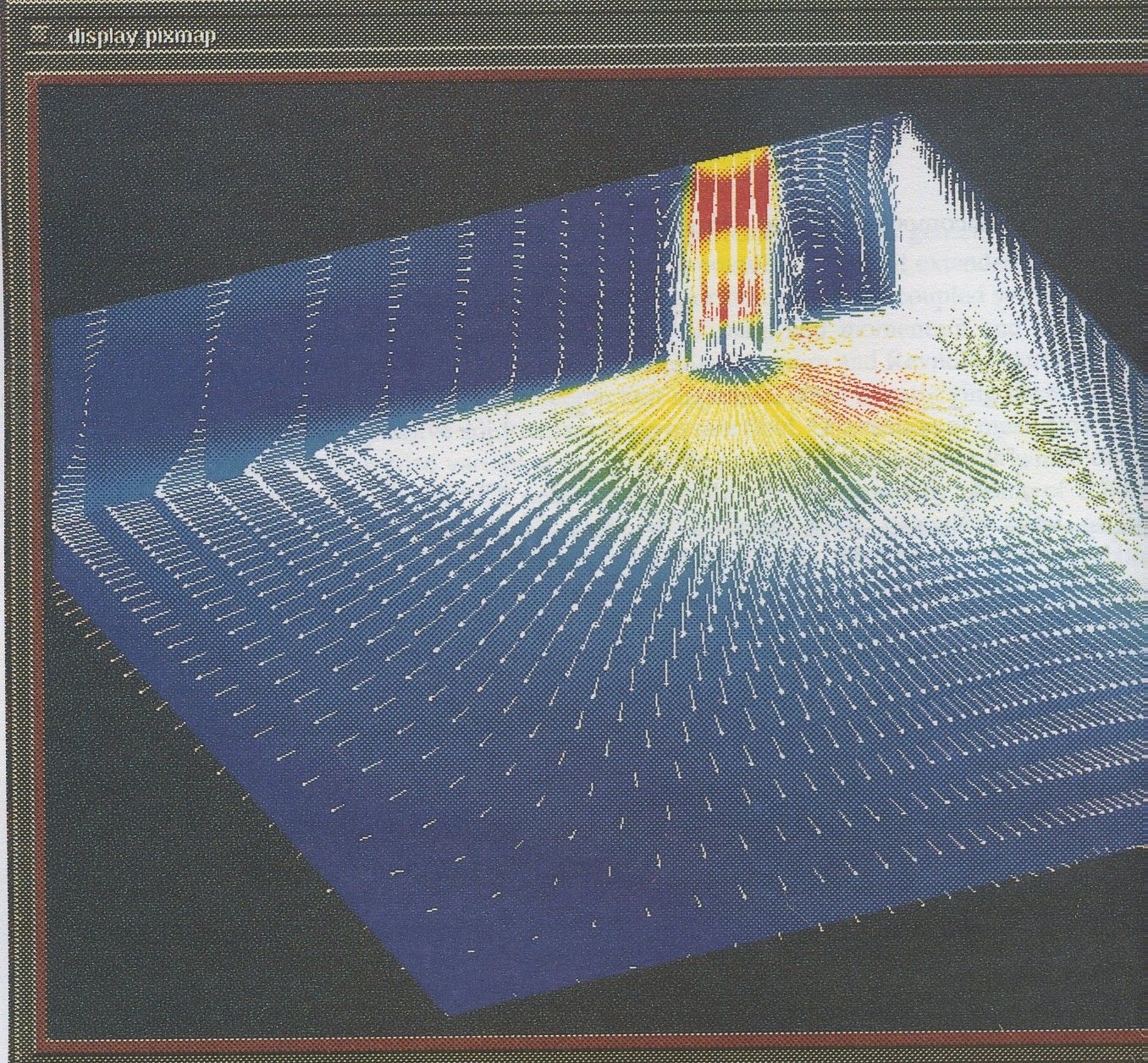
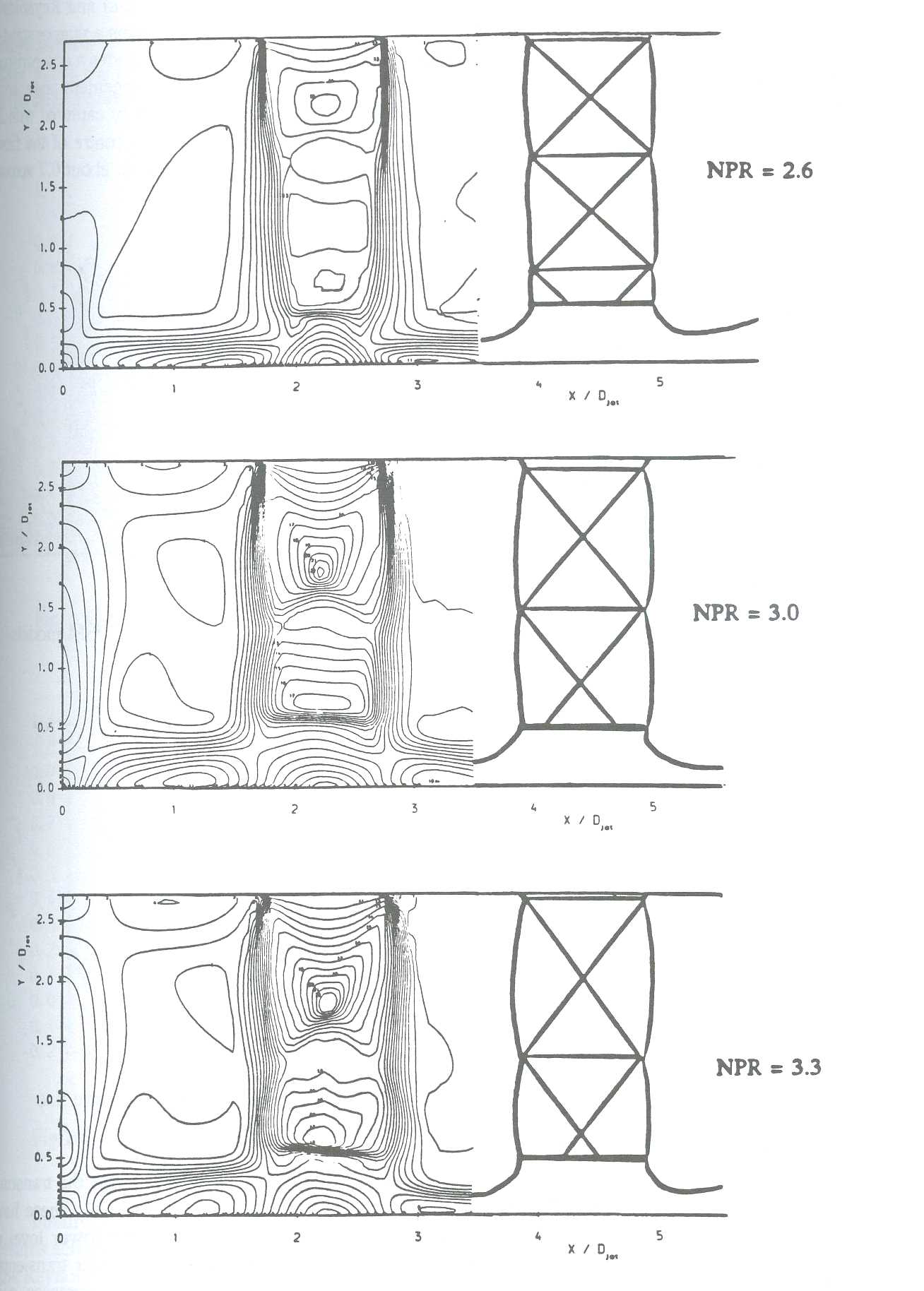
Fig. 7 compares the Mach-contour fields predicted with the eddy-viscosity (k-Ε) and Reynolds-stress models at NPR=3.3, and these serve to illustrate that the latter model returns a sharper standoff shock - a difference that is brought out particularly well in Fig. 8 which provides a comparison of static pressure variations along the jet axis. The origin, at Y=0, is the impingement plate, and the triangular symbols identify grid-line positions. As seen, the shock is credibly captured with 2 or 3 internodal distance. The maximum Mach number, 2.2, is reached in the centre of the first shock cell, while that just ahead of the stand-off shock is about 1.7, reducing to about 0.7 across the shock.
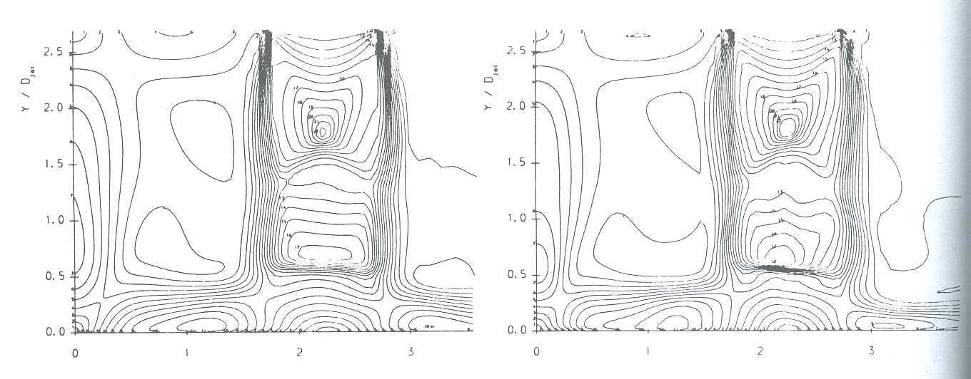
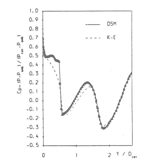
An important outcome of this part of the study has been the suggestion that the transonic jets feature periodic oscillations induced by instabilities in the impingement shock. These have been resolved only by the Reynolds-stress model which returns a significantly lower level of turbulence transport, thereby encouraging the revelation of non-turbulent (i.e. regular transients). The eddy-viscosity model, in contrast, over-estimates viscous transport and suppresses such oscillations. An impression of the intensity of time dependence is conveyed by Fig. 9. This shows predicted variations of impingement-plate pressure in comparison with experimental data for NPR = 3.0. The r.h.s. plot (b) shows solutions returned roughly at the extrema of oscillation, while plot (a) arises from the k-e model. Fig. 10 gives similar pressure-plots for NPR = 2.6 and 3.3, pertaining roughly to the mid-point of oscillation. Agreement with experiment is generally satisfactory for both models, but it must be recognised that the impingement and, perhaps to a lesser extent, the fountain-base pressure are largely dictated by convection processes, as opposed to diffusive transport.
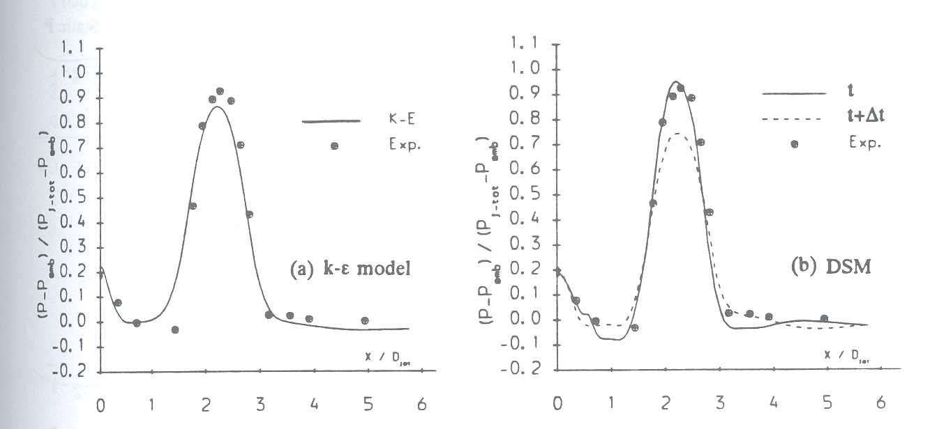
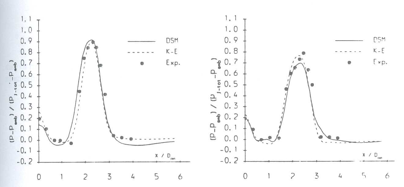
Finally, comparisons between predicted and experimental variations of static and total pressures across two fountain traverses at NPR = 3.0 are shown in Fig. 11. Any figure pertaining to the Reynolds-stress model includes two sets of curves reflecting solutions at oscillation extrema and identifying the sensitivity of the fountain structure to shock oscillations. As seen, the level of sensitivity is high, and this poses obvious difficulties in assessing model performance by reference to the experimental data. The comparisons suggest, albeit vaguely, that the Reynolds-stress model returns a somewhat wider, less pointed fountain than that arising from the eddy-viscosity model; this behaviour is also observed for other NPR values, and is qualitatively consistent with that found in the incompressible jet.
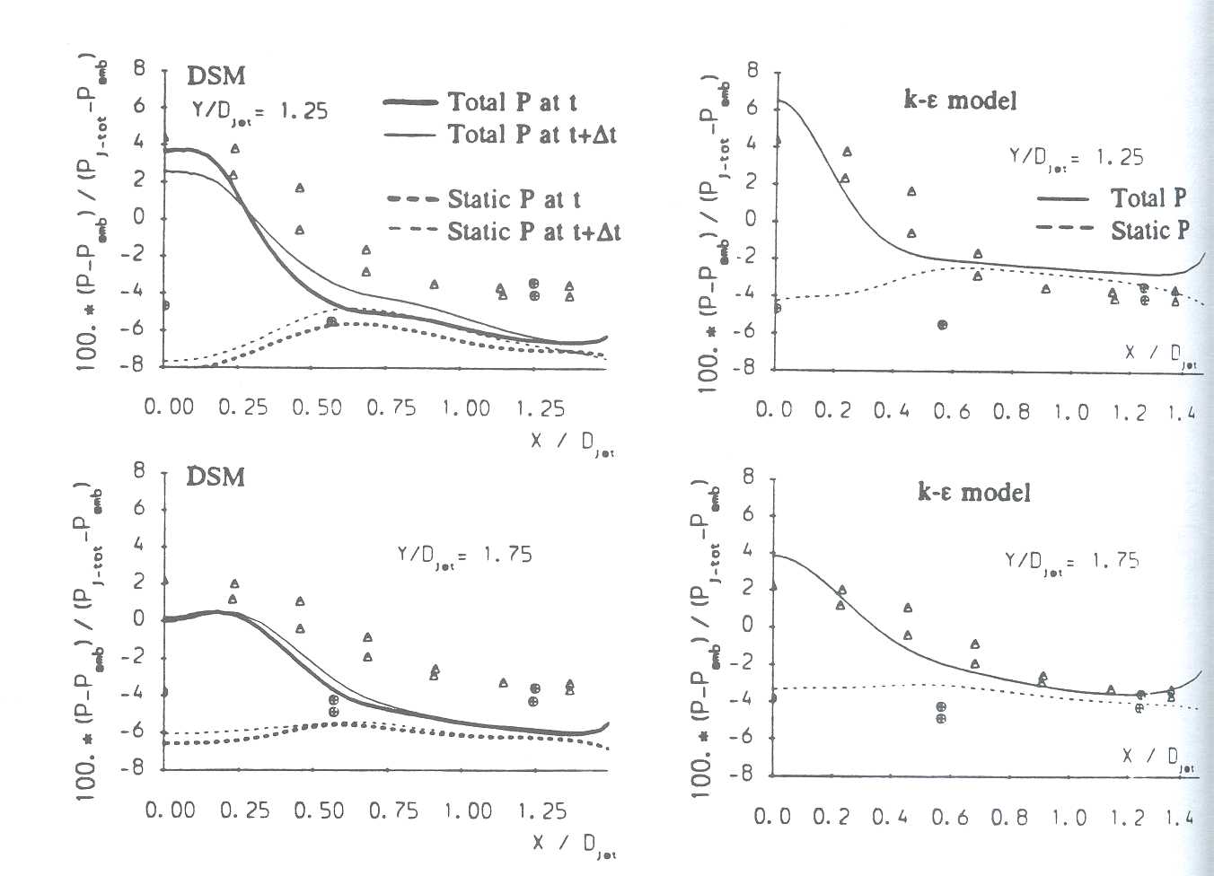
At the time of writing, computational studies continue for transonic jets in an effort to gain insight into the physical mechanisms provoking the oscillations and to obtain time-mean characteristics by integration over several oscillation periods.
1. Ince, N.Z. and Leschziner, M.A., "Computation of three-dimensional jets in crossflow with and without impingement using second-moment closure", Engineering Turbulence Modelling and Experiments, (Rodi and Ganie eds.), Elsevier, p. 143, 1990.
2. Ince, N.Z. and Leschziner, M.A., "Calculation of single and multiple jets in cross-flow with and without impingement using Reynolds-stress-transport closure", Paper 23.1, AGARD Symposium on Computational and Experimental Assessment of Jets in Cross Flow, Winchester, UK, 1993.
3. Ince, N.Z. and Leschziner, M.A., "Second-moment modelling of incompressible impinging twin jets with and without crossflow", Proc. 5th Int. IAHR Syps. on Refined Flow Modelling and Turbulence Measurements, Paris, 1993.
4. Ince, N .Z. and Leschziner M.A., "Second-moment modelling of subsonic and Transonic impinging twin jets", Royal Aero Soc. 1993 European Forum on Recent Developments and Applications in Aeronautical CFD, Sept. 1993, Bristol.
5. Lin, C.A. and Leschziner, M.A., "Computation of three-dimensional injection into swirling flow with second-moment closure", Proc. 6th lnt. Conf. on Numerical Methods in Laminar and Turbulent Flows, Swansea, pp. 1711-1725, 1989.
6. Saripalli, K.R., "Laser-Dopler velocitemer measurements in 3D impinging twin-jet fountain flows", Turbulent Shear Flows 5, (F. Durst, B.E. Launder, F.W. Schmidt and J.H. Whitelaw eds.), Springer, pp. 146-168
7. Abbott, W.A. and White, D.R., "The effect of nozzle pressure ratio on the fountain formed between two impinging jets," Royal Aerospace Establishment Technical Memorandum, P1166.
With the advent of supercomputers such as Cray Y-MP, flow dynamics problems are now amenable to solution by direct numerical simulation (DNS). The DNS method solves the full Navier-Stokes equations without turbulence modelling. The solutions obtained can provide spatially and temporally accurate information about the true physics of the flow without the interference of any empirical inputs. Because of its need to resolve all the scales of (turbulent) motion accurately, DNS requires the use of spectral or very high order finite difference methods, which are computationally demanding.
Much of work involving DNS has been with the incompressible flows at relatively low Reynolds number, notably the simulation of turbulent boundary-layer flow at a momentum thickness Reynolds number of 1410 (Spalart, 1988) and the simulation of transition to turbulence in channel flow at Reynolds number 5000 (Gilbert, 1988). Recent efforts have been focused on compressible flows. While this may mean simpler treatment of the incompressibility condition, it brings large number of extra terms in the equations to be solved. This makes implicit treatment of the viscous terms numerically expensive. As a result, certain spectral methods, such as Chebeshev, are no longer unsuitable. As an alternative, Sandham & Reynolds (1991) used a combination of a spectral method and high-order Pade schemes developed by Lele (1990) at NASA-Ames, and successfully simulated the compressible mixing layers. The aim of the present project is to extend the method to compressible shear layers in a round jet.
Little is known about the transition and turbulence in a round jet despite many experimental studies in this areas. However, understanding of such phenomena is very important, firstly because the sound generated by vortices in the initial shear layer is a significant component of the sound generated by a jet engine. Secondly, the combustion process in a jet engine is predominantly mixing controlled so increased mixing efficiency may lead to enhanced fuel economy. Because of the nature of the method, DNS is an ideal tool for providing more fundamental understanding of transition and mixing in a round jet.
Work to date has focused on the development and testing of a new DNS code for solving the full compressible Navier-Stokes equations for shear layers with variable Mach, Reynolds, Prandtl and Schmidt numbers as well as options for spanwise symmetry. A new Pade boundary formation has been incorporated based on recent numerical analysis. Considerable effort has been expended to make the code as efficient as possible on the Cray Y-MP. The code is now fully vectorised on the Cray Y-MP, the Mflops achieved being 160 or even higher depending on the mesh size. The validation of the code has been achieved by comparison with linear stability analysis and with previous mixing layer simulations. Simulations have then been performed to study the transition to turbulence in a compressible mixing layer with convective Mach number 0.8. Three Reynolds numbers ranging from low to medium were used. The initial disturbances were a pair of equal and opposite oblique waves. The simulation was carried out through the nonlinear stages to the formation of small scales and breakdown to turbulence. At time t = 36, Λ-vortices had formed out of the initial disturbance. Figure 1 shows this structure by plotting the pressure surface in three dimensions. The low pressure regions should correspond to the vortex cores. Similar vortex structure has been observed in experiments and simulations with different flow conditions. Later, the flow undergoes formation of high shear layers above the Λ-vortex, shear-layer roll-up and final breakdown to turbulence. Figure 1 shows the pressure field after transition. The presence of small-scale structures is evident. The colour contour plot in the background shows the passive scalar field. The picture is very much like those observed in fully developed turbulent flow in the flow visualisation of Clement (1991). The detailed discussions of these results are to be found in our papers (Luo & Sandham, 1994 a,b ).
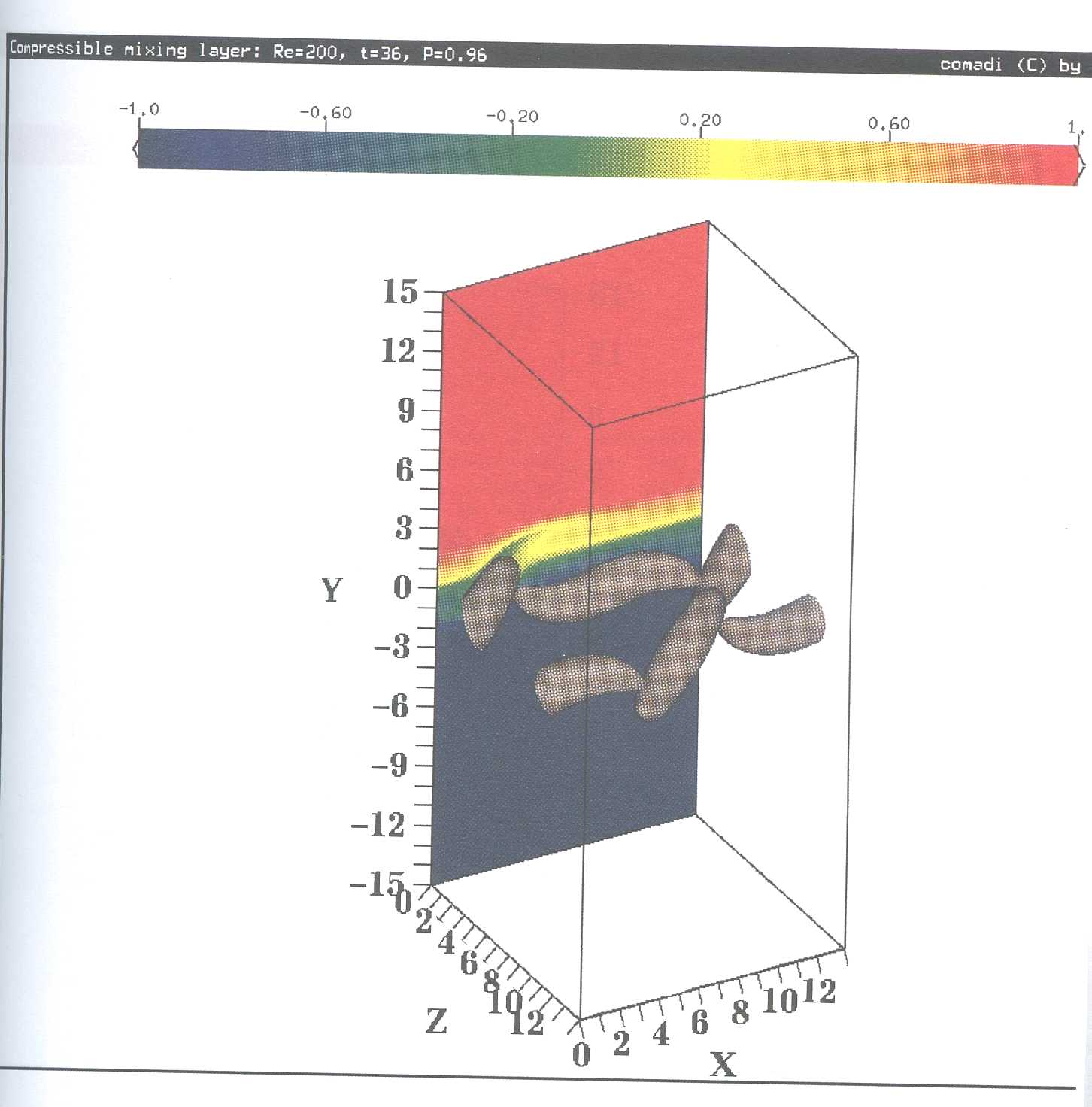
The main findings of these simulations are:
Clemens, N. T. 1991 An experimental investigation of scalar mixing in supersonic turbulent shear layers. Rep. T-274. High Temperature Gasdynamics Laboratory, Mechanical Engineering Department, Stanford University.
Luo, K.H. and Sandham, N.D. 1994a On the formation of small scales in a compressible mixing layers. The First ERCOFTAC Workshop on Direct and LargeEddy Simulation, Surrey, UK. March 1994.
Luo, K.H. and Sandham, N.D. 1994b Direct simulation of scalar mixing in compressible shear layers in transition. Fifth European Turbulence Conference, Siena, Italy, July 1994.
Sandham, N. D. and Reynolds, W. C. 1991 Three-dimensional simulations of large eddies in the compressible mixing layer. J. Fluid Mech. 224, 133-158.
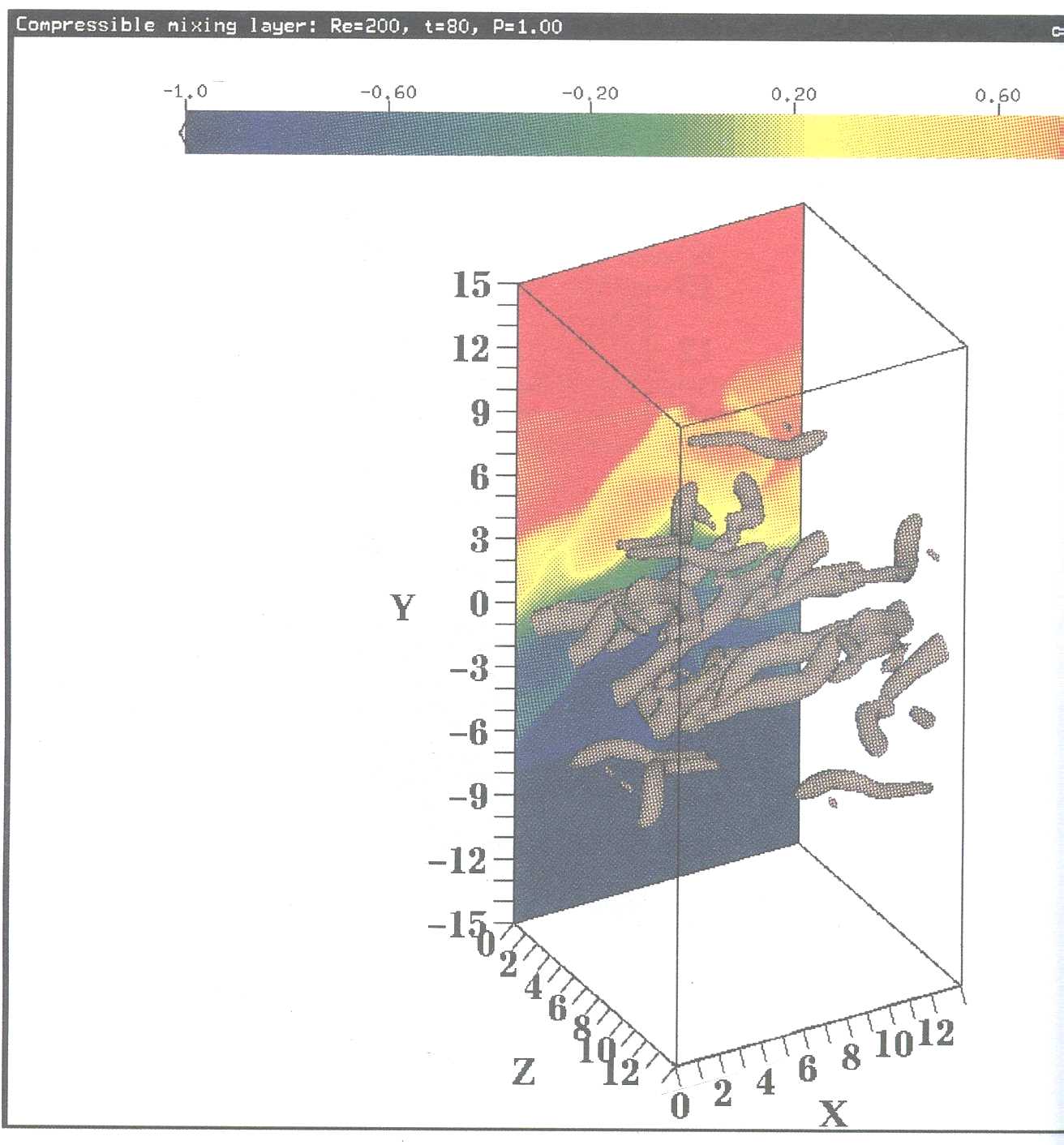
This brief report documents the use of the Rutherford CRAY YMP, under NERC Grant No GR3/8175A, during the months May-July 1993. The Grant was awarded to study stratified flow over hills, modelled by the incompressible Navier-Stokes equations with simple turbulence modelling. In view of possible unsteadiness in the flow and the presence of propagating waves, the unsteady equations are used, resulting in computations which are very time-intensive.
It was readily apparent from initial runs with the two-dimensional version of the code that the vector architecture of the CRAY was being utilised very inefficiently. The cpu-time gain over the SUN Sparc 2 was only by a factor of around 4.5. The corresponding factor for the three-dimensional code was around 2.3. (Several changes had been made in the structure of the three-dimensional code and presumably even less vectorisation was possible.) Inclusion of compiler options to invoke automatic vectorisation yielded negligible improvement. Vectorising the code was therefore seen as a priority, but in view of the work involved and the time constraint (the Grant period expired in September) this could not be done immediately.
Because of the long running times required for the three-dimensional code (40hrs approx), a typical computation was divided up into several shorter runs. At the end of each run a dump of the solution would be made, which was then read in and used to continue the computation. Two types of jobfile were set up: one to control a run starting from specified initial conditions, and the other controlling a run starting from a dump. In view of their size, the flow dumps were stored on the CRAY itself. Graphical output was also dumped periodically, which was sent back to our local SUN workstations for plotting. In order to be read by the SUN the graphical data had to be formatted, and large files were created (up to 8mb). These were also stored temporarily on the CRAY and were transferred using ftp from our workstation. Small output files containing diagnostic data were sent to the IBM via the Reader. This involved setting up a minidisk on the IBM dedicated to receiving output from the CRAY. These files could then be transferred back to our workstation using rtransfer.
Of our cpu allocation of 100hrs, approximately 80hrs were used. Two computations of flow over a three-dimensional cosine hill were performed, at Froude numbers of Fh = 0.7 and Fh = 0.6, and up to nondimensional times of 100 and 75 respectively.
These are roughly the towing-times of corresponding experimental studies (Castro & Snyder, 1993). In the light of these experimental results, we were expecting regions of wave-breaking and secondary separation to occur in both computations, with the two regions merging at the lower Froude number. This was indeed the case. Fig 1 shows velocity vectors from the two computations, at a nondimensional time of 20, with clear merging occurring at Fh = 0.6. These results are believed to be the first numerical computations of such a merged flow. Full details of all aspects of the computations can be found in Paisley (1993) and Paisley & Castro (1993).
The CRAY YMP has been used to compute three-dimensional time-dependent density-stratified flows over hills. Results have been obtained which agree well with experimental data and which contain features not previously seen in numerical computations. Further computational work is planned to investigate the effects of parameters such as hill-shape, Froude number and flow shear. Further applications for time on the CRAY are being made and work is in hand to vectorise the code. Inclusion of numerical techniques such as multigrid and grid-nesting to improve the efficiency of the solution process is also planned.
Castro I P & Snyder W H 1993 Experiments on wavebreaking in stratified flow over obstacles. I.Fluid Mech. 255, 195-211.
Paisley M F 1993 Stratified airflow over mountains. Dept.Mech.Eng. Report No. 09/93, Surrey University.
Paisley M F & Castro I P 1993 Numerical experiments on wave-breaking in stratified flow over hills. In preparation.
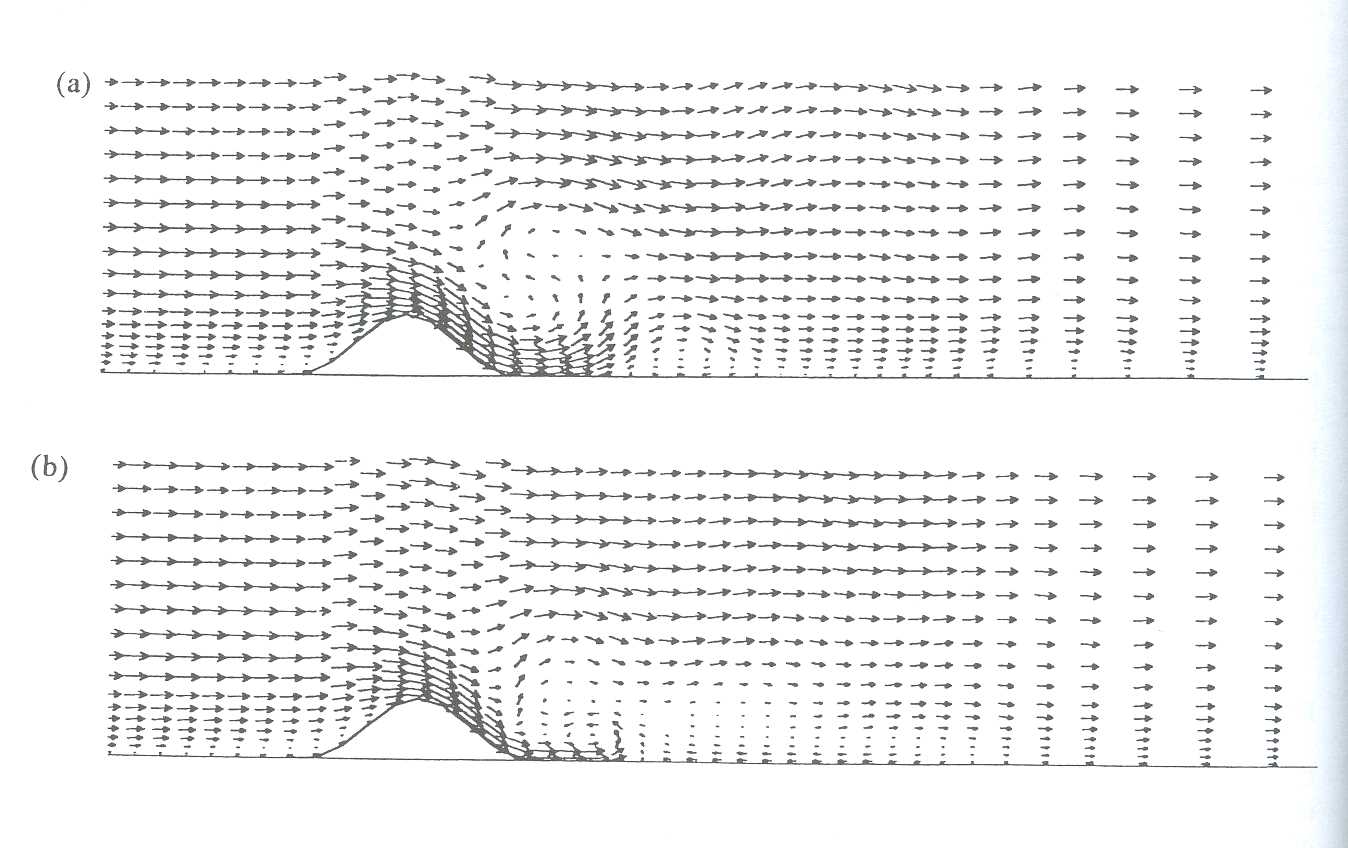
Over the past two years numerical and analytical studies have been carried out on viscous flow stability, with the numerical work carried out on the Cray X-MP at RAL under grants GR/G28826 and GR/H82259. Three different areas were considered:
A sophisticated pseudo-spectral code was used to track the growth of non-linear Tollmien-Schlitchting waves in a two-dimensional subsonic/incompressible flow governed by the unsteady interactive (triple deck) boundary-layer equations. The solution to such a problem can break down in a finite time due to the development of a singularity, and some knowledge of the structure of the singularity in required in order to reformulate the problem and follow the growth of the disturbance at a greater magnitude.
In this study the behaviour of the Fourier coefficients was analysed to investigate the terminal nature of the singularity, and the numerical results were then compared with those from a possible theoretical singularity structure. There was a measure of agreement, particularly with regard to the wave speed of the singularity, but also some significant disagreements.
Two-dimensional Navier-Stokes flow in non-uniform channels where large scale instabilities in the flow are forced by an unsteady mass flow is of considerable interest as the resulting large scale motions can enhance mixing rates in the vessel and heat transfer to and from the vessel walls, and significantly affect the force exerted by the fluid on the vessel walls.
For a stepped channel with an oscillatory mass flow rate, the effects of varying the Reynolds number, the Strouhal number, and the size of the step were examined numerically. A strong 'vortex wave' can be generated during the forward phase when the flow is over the step into the expansion, with the peak values of the forces on the wall much greater than those in steady flow with the the same Reynolds number. Secondary effects can result in a complex flow pattern with each major structure of the flow consisting of an eddy with more than one core. No vortex wave was found during the reverse phase when the flow was into the constricted part of the channel. In addition, a theoretical model for wave generation for unsteady flow in a non-uniform channel was developed. The model has limited application to and agreement with the full Navier-Stokes solutions.
A further study of pulsatile flow in a channel with a bump on one wall forming an asymmetric constriction was performed. Again a strong vortex wave was generated, and it was found that the pattern of the wave is significantly affected by the form of the imposed flow rate.
Work is continuing in this area, currently focusing on flow in a channel with slightly nonparallel walls downstream of a step.
It is well known that if the width of a two-dimensional channel increases gradually with distance downstream, a steady flow will separate for values of the Reynolds number above a rather moderate critical value. Further, the separated flow is non-unique: even when the geometry is symmetric, so that a symmetric separated solution exists, the flow is generally asymmetric, clinging to one wall or the other. A series solution method was used to investigate the process of separation and the development of asymmetry in the solution by adding the inertial contribution to the cross-stream pressure gradient to the boundary-layer problem. In addition, calculations were performed for the standard symmetric boundary-layer problem, and for Navier-Stokes flow in an gradually expanding asymmetric channel. The results from the different methods were generally consistent. For the Navier-Stokes problem multiple solutions were found: the preferred solution has the initial separation on the curved wall, but at least one other solution, with separation on the straight wall, exists.
Tutty, O.R. Pulsatile Flow in a Constricted Channel. Trans ASME: J. Biomech. Eng., 114, 50-54 (1991).
Tutty, O.R. & Pedley, T.J. Oscillatory Flow in a Stepped Channel. J. Fluid Mech., 247, 179-204 (1993)
Tutty, O.R. & Pedley, T.J. Unsteady Flow in a Non-uniform Channel: a model for wave generation. Phys. Fluids A, 6(1), l0pp (1994).
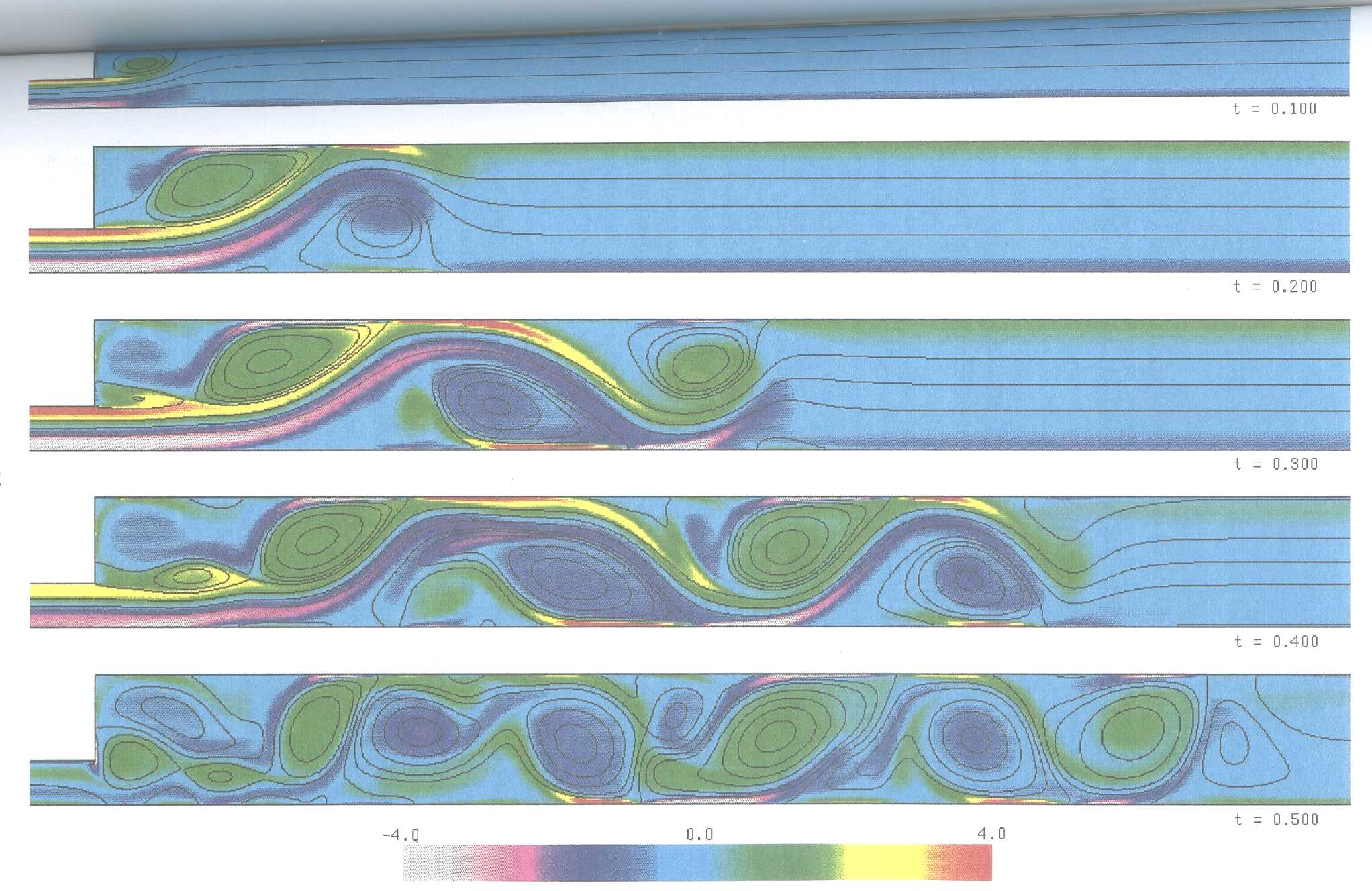
Two non-linear finite element programs have been restructured by using vectorization techniques in order to run efficiently on the Cray X-MP /416. One of them has also been multi-tasked to take advantage of the four processors of the machine. The techniques used in restructuring the software are discussed, and it is shown that each program must be treated individually. The resulting speed enhancements are shown to be program dependent, with a speed-up of approximately 20 being achieved with one of the programs.
Non-linear finite element analyses generally require a large amount of CPU time and memory. Supercomputers, such as the Cray X-MP/416, are well suited for such tasks. However, a program which is written for conventional scalar computers will not perform well on a multi-processor vector machine. Special programming techniques are required in order to take full advantage of a supercomputer architecture.
This paper discusses the implementation of vector processing and parallel processing techniques in two non-linear finite element programs running on the Cray X-MP/416. One program is called TOMECH, which has been developed as a research tool for the study of plasticity and fracture [1] and has recently been extended to analyze the microstructural processes of void nucleation, growth and coalescence in ductile materials and components under increasing loads [2]. The Newton-Raphson iteration scheme is used in this program to obtain the non-linear solutions at each successive loading increment. The other program is called DAMAGE XX, which analyses the high temperature creep deformation and rupture of structural components using Continuum Damage Mechanics (CDM) [3, 4]. Since the deformation progresses in real time, a Runge-Kutta procedure is used to solve the initial value boundary problem. The emphasis in this paper will be put on the vectorization and parallization of DAMAGE XX.
To vectorize a program simply involves the writing of mathematical algorithms so that long lists of numbers are manipulated together rather than one by one [6]. There is usually no unique vectorization of any particular task. The experience gained in this research shows that successful vectorization of a task generally meets the following requirements: 1. an optimal algorithm with the least possible number of operations for the given task; 2. the use of long vectors; 3. the use of memory accessing modes with small memory accessing stride in most vector mode operations, which provides less chance of memory conflict.
However, it should be stresses at this point that the research reported here concerns only the CRAY architecture and the techniques are not necessarily transferable to other computers. For example, the vectorizing of inner DO loops; and, making extensive use of indirect addressing ( i.e. X(J(I))) are features which can be used with advantage on the CRAY. On the other hand, some features are common such as small memory strides which are even more important in computers (e.g. workstations) that rely on small fast 'cache' memories.
DAMAGE XX deals with plane stress, plane strain and axi-symmetric problems and it employs constant strain 3-noded triangle elements. As a program aimed at modelling creep deformation and rupture, creep strain, stress, and damage are integrated with respect to time t from the elastic state, based on the following constitutive equations:
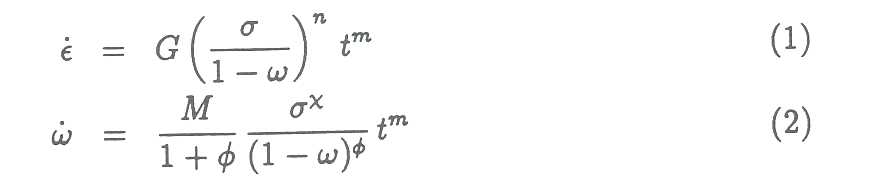
where ![]() is the creep strain rate,
is the creep strain rate,
![]() the creep damage rate, σ the stress; and m, n, G, M, Φ, ψ are
material constants. The integration is carried out over a series of discrete time steps
using a fourth-order Runge-Kutta technique; the procedure involves the repeated
solution of the boundary value problem to determine the field quantities required
for the numerical integration. Creep damage w develops monotonically in time throughout
the structure, and failure of an element is deemed to have occurred when the state
parameter attains a prescribed value. The problem is then redefined and the time
integration is continued taking the field variables as the new starting point.
The whole procedure requires evaluation of creep damage rates, of incremental
displacements, and of creep strains and
stresses at every iteration. The solution routine is thus accessed frequently.
In fact, four subroutines conducting these functions have been found, by using
the Cray performance monitor, FLOWTRACE [5], to be the core time consuming parts
in DAMAGE XX. These subroutines are EDISP, ESTRES, ECSWLD and BANA.
Vectorization of them are discussed in detail here.
the creep damage rate, σ the stress; and m, n, G, M, Φ, ψ are
material constants. The integration is carried out over a series of discrete time steps
using a fourth-order Runge-Kutta technique; the procedure involves the repeated
solution of the boundary value problem to determine the field quantities required
for the numerical integration. Creep damage w develops monotonically in time throughout
the structure, and failure of an element is deemed to have occurred when the state
parameter attains a prescribed value. The problem is then redefined and the time
integration is continued taking the field variables as the new starting point.
The whole procedure requires evaluation of creep damage rates, of incremental
displacements, and of creep strains and
stresses at every iteration. The solution routine is thus accessed frequently.
In fact, four subroutines conducting these functions have been found, by using
the Cray performance monitor, FLOWTRACE [5], to be the core time consuming parts
in DAMAGE XX. These subroutines are EDISP, ESTRES, ECSWLD and BANA.
Vectorization of them are discussed in detail here.
Globally, the lengths of the working vectors in DAMAGE XX have been maximized to enhance the performance of vector processing. In the finite element method, basic variables, such as stress, strain, displacement and damage rate, are based on elements, so that the lengths of working vectors are usually limited in an element. In the original DAMAGE XX program, for example, the lengths of the working vectors for stress and strain were four, and that for displacement was six. By writing out explicitly some of DO-loops with short lengths the lengths of working vectors may be increased to the number of unfailed elements, NUNF, or multiples of it in most situations. In doing this, a vector which maps the unfailed elements to the original elements has been introduced. This vector is accessed in the program frequently.
All the subroutines in DAMAGE XX have been examined and vector processing has been enabled on most of the DO-loops in the program. In particular, high speed for the following core subroutines has been achieved.
EDISP: In this subroutine, nodal creep forces are calculated from the accumulated creep strains ee by using the following equation
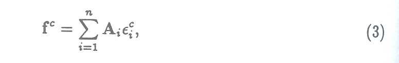
where n is the number of unfailed elements; and Ai= ∫vi Bt iD dv, vi denotes the volume of the ith element, D is the matrix of elastic constants. Bi is calculated from the shape function Ni [8]
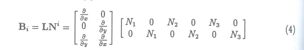
where L is the linear operator and Nj, j = 1,2,3 are the components of the shape function Ni. Therefore, the contribution of the ith element to fc is
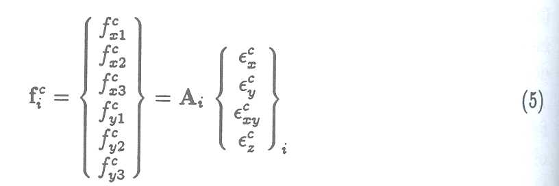
where Ai is a 6 × 4 matrix; fc xj, j = 1,2,3 denotes the creep force in the x direction at the jth node and fc yj, j = 1,2,3 denotes the creep force in the y direction at the jth node. To vectorize this subroutine, terms involved in calculation of each component of fc i were written explicitly. Two vectors with length of three times the number of elements were introduced to store the nodal creep forces of all the elements to avoid the data dependence, or concurrence, in the vector processing. These forces were then added to the global nodal force vector to evaluate the nodal displacements by calling the matrix solution subroutine BANA.
ESTRES: In this subroutine, the total strains and stresses are calculated. The total strains in the ith element are computed by using
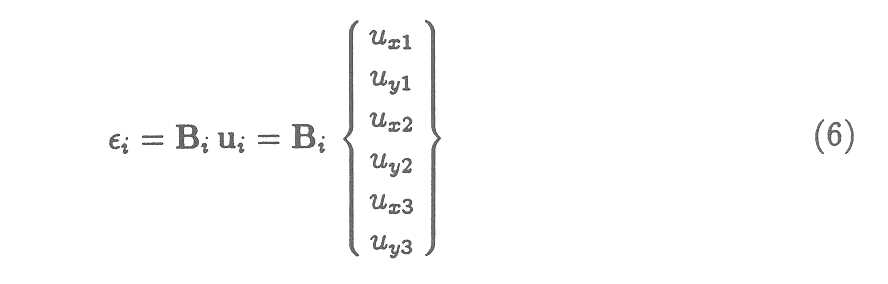
where ui, is the displacement vector of the nodes in the ith element. Explicitly writing out all terms in the calculation of each component of the total strain Εi enables the vector processing over the length NUNF. The same technique was used in calculation of stresses in this subroutine.
ECSWLD: This subroutine evaluates the creep strain rate and the damage rate over all unfailed elements according to equations (1) and (2). In this subroutine, all DO-loops with short vectors were replaced by those with vector length equal to NUNF. General optimization techniques, such as loop unrolling, loop jamming, segmentation of a non-vectorization loop, inversion of nested loop and so on [5, 9, 10], were used whenever possible to eliminate vector inhibiting conditions, and to improve the performance. Additional COMMON blocks were introduced to store those elemental materials parameters which are used frequently, and which were originally calculated repeatedly.
BANA: In this subroutine, the Cholesky method is used to solve the equations:

where K is the global stiffness matrix, U the nodal displacement, F the external loads, Fc the creep force. The K matrix was stored diagonally in a one-dimensional vector Z. To get better vector performance, this was re-arranged so that the elements in K were placed row by row in Z, which reduces the memory accessing stride from the half-band width to 1 for forward substitution. On the other hand, a slightly different method, the Triple-Factoring method [6] was used to replace the Cholesky method, which has less operations [6], especially for vector processing.
To assess the speed-up of individual subroutines due to the re-writing, an example was used which had 156 nodes and 261 elements and run for 226 iterations under vector mode. Listed in Table 1 are the cpu times which were spent on each subroutine before and after the re-writing.
Table 1. Speed-up of Subroutines
| Subroutine | CPU time (Sec) before re-writing |
CPU time (Sec) after re-writing |
Speed-up |
|---|---|---|---|
| EDISP | 8.6017 | 1.1349 | 7.6 |
| ESTRES | 5.6931 | 1.0483 | 5.4 |
| ECSWLD | 19.9436 | 1.4124 | 14.0 |
| BANA | 8.4242 | 3.1334 | 2.7 |
The overall speed-up of the program by vectorization may be demonstrated by two examples. In the first, there are 637 elements and 350 nodes. In the second, there are 1374 elements and 747 nodes. In Table 2, the CPU times of the new version running in vector mode are compared with those of the old version running in scalar mode and that in vector mode respectively. The number of Floating Point Operations in Megaflop units, and the speed in Megaflop/s (Megaflop units per second) for each run are also listed in Table 2. It can be seen that the overall speed-up comes from two factors. One is the reduction of the number of operations and the other is the increase of the speed. The former is mainly due to the optimal selection of algorithms; while the latter is due to the correct vectorization. It was found that in all cases there are more than 98% operations in the new version of DAMAGE XX running in vector mode.
| No. | Old (Scalar mode) | Old (Vector mode) | New (Vector mode) | Speed-up | ||||||
|---|---|---|---|---|---|---|---|---|---|---|
| time | Mflop | Mflop/s | time | Mflop | Mflop/s | time | Mflop | Mflop/s | ||
| 1 | 929.2 | 9190 | 9 | 645.4 | 13985 | 21 | 79.0 | 6676 | 84.5 | 11.8 |
| 2 | 420.8 | 4326 | 10 | 253.2 | 6791 | 26 | 28.7 | 2155 | 74.9 | 14.6 |
When TOMECH is used to study plasticity and fracture problems, the Newton-Raphson iteration scheme is used to obtain the non-linear solutions at each loading increment, during which the stiffness matrix is re-evaluated and decomposed at a frequency whose value is controlled by the user. By using the Cray performance monitor FLOWTRACE[6], it was identified that the formation of the stiffness matrix and the inverse of the global stiffness equations were the most intensive computing stages for large problems. Vectorization of the program was, therefore, concentrated on these two parts.
The basic operations in forming the stiffness matrix of each element are formation of the B matrix from the element shape function[7], and the computation of the element stiffness matrix
where D is the elasticity matrix. For a 20-noded element, the dimensions of D and B are 6 × 6 and 6 × 60 respectively. The calculation of an element stiffness matrix is usually completed by using several nested DO-loops with logical operations to point to the position of an element in vectors. This is inefficient in vector operation.
The first step in vectorizing this part of the code was to arrange the calculation in one-dimensional loops with every DO-loop running in vector mode and to eliminate logical operations inside them. The process may be demonstrated by considering a 20-noded 3-dimensional element as an example and by assuming that D × B = A has been completed, where A is a 6 × 60 matrix. The question is then how to evaluate ki(I,J) efficiently, I=1, ... ,60; J=l, ... ,60. Since ki is symmetric, only those elements in its upper triangle need to be calculated. These elements were stored in a one-dimensional vector S(I),1=1, ... ,1380 so that S(1)=ki(1,1); S(2)=ki(l,2), S(3)=ki(2,2); S(4)=ki(l,3), S(5)=ki(2,3), S(6)=ki(3,3); .... ;.. , S(l379)=ki(59,60), S(1380)=ki(60,60). A constant pointer ISTT(I),I= 1,...,1380 was used to indicate the corresponding column number in ki for a given element S(I). The integration within ki is performed by the following codes
      DO 10 I=1,1380
      J=ISTT(I)
      K=I-(J*(J-1))/2
      S(I)=S(I)+ WJG*(B(1,K)*A(1,J)+B(2,K)* A(2,J)+
     1     B(3,K)*A(3,J)+B(4,K)*A(4,J)+
     2     B(5,K)* A(5,J)+B(6,K)* A(6,J))
 10   CONTINUE
where WJG is the weighting factor. Note that the unrolling technique[8,9] is used to accomplish part of this. The vector length for this operation is 1380 while the minimum memory accessing strides were used for all three vectors, A,B and S.
This algorithm has proved to be very efficient. Bench mark tests showed that the CPU time consumed in this stage was 10-13 times less than that of the original codes running in vector mode. The exact value depends on the size of the problem. However, the use of the indirect addressing vector ISTT(I) is known to be efficient on the CRAY, but not on some other vector computers.
The solution stage of the program was reviewed by comparing various algorithms and selecting the most efficient using a set of bench mark tests. Techniques for improving the performance of vector operations [6,8,9] were applied whenever possible.
There are currently four different algorithms available in TOMECH: the Cholesky method (CHOL), Crout's method (CROU),the Incomplete Cholesky-Conjugate Gradient method (ICCG), and the Evans Preconditioned Conjugate Gradient method (EPCG). For large problems, the ICCG and the EPCG methods are the only ones available due to the limit of memory space on the computer. These two methods, particularly, the ICCG method, were studied in detail. Some of the code was re-written to enhance the vector performance, and Cray directives [6] were introduced in some instances to enable vector processing to occur, which was otherwise inhibited.
The overall speed-up of the program due to vectorization varies with the size of problem. General speaking, for a large problem of more than 10 000 degrees of freedom, the new version runs about 3-4 times faster than the original version running in vector mode, disregarding the CPU time consumed in mesh generation. This enhanced performance made it possible to conduct a comprehensive study on the numerical modelling of the damage process in ductile materials [11], using the limited computer resource available.
Parallel processing on the CRAY X-MP /416 is handled by three modes of multitasking: Macrotasking, Microtasking, and Autotasking. Macrotasking supports parallelism at the subroutine level. Task creation, synchronization, and communication are specified explicitly by the programmer using subroutine calls. Microtasking works at the statement level. It makes use of compiler directives inserted by the programmer. These directives are given to a preprocessor which generates subroutine calls for the creation of parallel tasks and their synchronization. Autotasking is similar to microtasking except that in autotasking parallel processing is started and ended at any number of suitable points within a subroutine; while the microtasking requires that parallel processing always starts at the first executable statement of a subroutine and always ends at the last executable statement of the subroutine. Due to the convenient nature of autotasking, this method was concentrated on in the multitasking studies.
The program DAMAGE XX has been implemented with autotasking directives to exercise this facility. On the CRAY X-MP /416, CMIC$ is used to indicate the multitasking directives in a Fortran program. One directive which has been used extensively in restructuring of the program is DOALL. This directive may be placed before those multi-taskable DO loops, where potential benefit due to multitasking exists, to initiate parallel processing. The end of the DO loop indicates the end of the parallel region. In DAMAGE XX, the most time consuming DO loops which have been studied for vectorization were candidates for multitasking. For example, in Subroutine ECSWLD, the effective stresses of each active element are required in the calculation of damage rate and so on. These quantities are computed in a separate DO loop and stored in a vector SEFF. This DO loop is multi-tasked by using the autotasking directive DOALL as follows
CMIC$ DOALL SHARED (NOK,NEUNF,SEFF,STRESS) PRIVATE(I,K,L)
CMIC$1      NUMCHUNK (4)
      DO 300 I=1,NOK
      K=NEUNF(I)
      L=4*K-4
      SEFF(I)=SQRT(STRESS(L+1)*STRESS(L+1)+STRESS(L+2)*
     1    STRESS(L+2)+3.0*STRESS(L+3)*STRESS(L+3)
     2    +STRESS(L+4)*STRESS(L+4)-STRESS(L+1)*
     3    (STRESS(L+2)+STRESS(L+4))-STRESS(L+2)*
     4    STRESS(L+4))
300   CONTINUE
where STRESS is the vector in which all stress components are stored element by element, and NOK is the number of elements which are still active. It may be noted that those parameters within the DOALL directive are required to define, for example, the scope of data (SHARED, PRIVATE), and the the number of chunks (NUMCHUNK) that the DO loop should be broken up into. In this example, NOK, NEUNF; SEFF, STRESS are variables shared by all processors; that is, they have one storage location that is accessible to all of the executing processors. I, K, and L are variables owned privately by each processor. That is, each task (or processor) will have its own private copy of the variables. The iteration space in the DO loop will be broken into 4 chunks of equal size (with a possible smaller residual chunk), in accordance with 4 processors of the machine. Since NOK is usually several thousands in size, the breaking up of the iterations does not very much affect the vector performance as shown by some of the experiments. The unrolling technique, for calculation of the effective stress of each element, is used here to improve the vector performance. Other parameters in this directive [12] may be used as well to exercise control on how the concurrent execution should be done.
There are cases that multitasking is the only way to improve the performance substantially. For example, when an element fails the global stiffness matrix must be re-formed. This requires calling subroutines to evaluate the stiffness matrix for each element. Vectorization in this case is not possible. However, as the calculation of the stiffness matrix of each element is independent of each other, multi-tasking can be achieved by using PARALLEL/END PARALLEL and DO PARALLEL/END DO directives [12] such as:
CMIC$ PARALLEL SHARED (NOK,NEUNF,K, .... ) PRIVATE(I,F,NOD, .... )
CMIC$ DO PARALLEL NUMCHUNK (4)
      DO 100 l=l,NOK
      L=NEUNF(I)
      .........
      pass the coordinates of nodes in element L to NOD
      .........
      CALL ELSTIF(NOD,F)
      .........
CMIC$ GUARD
      CALL PAKB(F,K)
CMIC$ END GUARD
 100  CONTINUE
CMIC$ END DO
CMIC$ END PARALLEL
where F is the element stiffness matrix which is private to each element, and K is the global stiffness matrix which is shared by all tasks. ELSTIF is the subroutine in which element stiffness is calculated, and PAKB is used to assemble each element stiffness matrix into the global stiffness matrix K. The directive pair GUARD/END GUARD is used to ensure that only one processor writes to the K matrix at any one time.
An example with 5301 elements and 2746 nodes, which gives 5492 degrees of freedom, has been used to assess the multitasking speed-up. Listed in Table 3 are the timing information of two typical runs. The first column shows the number of processors used in each run, The second and the third column give the CPU time and Wall clock time in seconds. The speed-up is calculated by dividing the wall clock time in multitasking environment by that of the same job running on single processor.
Table 3. Speed-up of DAMAGE XX by multitasking
| NCPUS | CPU time (Sec.) | Wall clock time (Sec.) | Speed-up |
|---|---|---|---|
| 1 | 151.20 | 153.26 | - |
| 4 | 170.24 | 97.78 | 1.57 |
Due to the fact that the LAPACK solver SPBTRS, which takes 40% of the cpu time in this example, can not be multi-tasked for single right hand equations, the speed-up of 1.57 is what one can achieved on four processors according to the Amdahl's law [12).
Because TOMECH has been developed as a research finite element program for the solution of a wide range of elastic-plastic problems, there are several types of elements and various options in the program to be set by the user. It is not possible to use the same techniques as were used in the vectorization of DAMAGE XX to extend the length of vectors in most of the DO-loops so that they are equal to the number of elements or the number of nodes. The size of TOMECH, about 35000 lines of code, limited the amount of analysis and restructuring of the whole program because the time available to do this was short. Hence it was not possible to achieve the speed-up attained with the shorter modularised code of DAMAGE XX. This suggests that in the writing of future finite element programs, it would be easier to achieve vectorization by using a modular structure. In each module, one specific problem should be solved, for example, plane strain using triangular elements.
Substantial speed-up can be achieved by vectorization for specific finite element programs. Even for large programs, such as TOMECH, a small effort in vectorization can result in considerable improvement in performance. Large problems, especially those requiring solution of many non-linear equations, which are otherwise almost impossible to solve [11, 13), can benefit mostly by restructuring of the programs.
The overall speed-up by vectorization and by multitasking for DAMAGE XX reaches around 20 times. This figure can be further increased if the equation solver can be multi-tasked. Currently, the LAPACK solver SPBTRS runs in vector mode very efficiently; while the fact that it cannot run on multiple processors limits the overall parallel performance of the program.
The authors gratefully acknowledge the support provided by the United Kingdom SERC, by Nuclear Electric, Berkeley Laboratories, and by CRAY U.K.; and also discussions with Dr. R.Evans, Dr. J.Reid and Dr. D.Nicholas of the SERC Rutherford and Appleton Laboratory, held during the course of the research.
[1] A.G.Dix, The TOMECH User's Guide, Sheffield University. 1991.
[2] B.A.Bilby, I.C.Howard, and Z.H.Li, "Seventh Report on the Stability of Crack in Tough Materials: Prediction of R-curves in Wide Plate Tests Using Simple Void Growth Theory and Preliminary Results on the Rousselier Damage Theory", Dept of Mech. & Proc. Eng., University of Sheffield, Feb. 1990.
[3] D.R.Hayhurst, P.R.Dimmer, and C.J.Morrison, Development of Continuum Damage in the Creep Rupture of notched bars, Phil. Trans. R. Soc. Lond., A311, 103-29, 1984.
[4] F.R.Hall and D.R.Hayhurst, Continuum Damage Mechanics Modelling of High Temperature Deformation and Failure in a Pipe Weldment, Proc. Roy. Soc. Lond. , A433, 383-403, 1991.
[5] "CFT77 Reference Manual", SR-0018 C, Cray Research Inc., 1986.
[6] P.Tong and J.N.Rossettes, "Finite Element Method, Basic Technique and Implementation", M.I.T. Press, Cambridge, Mass., London, 1977.
[7] E.Anderson, Z.Bai, C.Bischof, J.Demmel, J. Dongarra, J. Du Croz, A.Greenbaum, S.Hammarling, A.McKenney, S.Ostrouchov, and D. Sorensen, "LAPACK Users' Guide", to be published by SIAM, 1992.
[8] O.C.Zienkiewicz, "The Finite Element Method", 3rd Edition, McGraw-Hill book Company Limited, London, 1977.
[9] J.J.Dongarra, "Redesigning Linear Algebra Algorithms", Mathematiques Informatique, No.l, 51-60, 1983.
(10] T.J.R. Hughes, RM.Ferencz and J.O.Hallquist, "Large-scale Vectorized Implicit Calculations in Solid Mechanics on a Cray X-MP /48 Utilizing EBE Preconditioned Conjugate Gradients", Computer Methods in Applied Mechanics and Engineering 61 215-48, 1987.
(11] Z.P.Wang, B.A.Bilby, I.C.Howard, and Z.H.Li, Numerical Study of Ductile Fracture on the Cray X-MP /416, to be published, 1990.
[12] "CRAY Y-MP, CRAY X-MP EA and CRAY X-MP Multitasking Programers Manual", SR-0222 F, Cray Research Inc., 1986.
[13] Z.P.Wang and D.R.Hayhurst, "Design of a Pipe Weldment Using Creep Continuum Damage Mechanics", to be published, 1992.
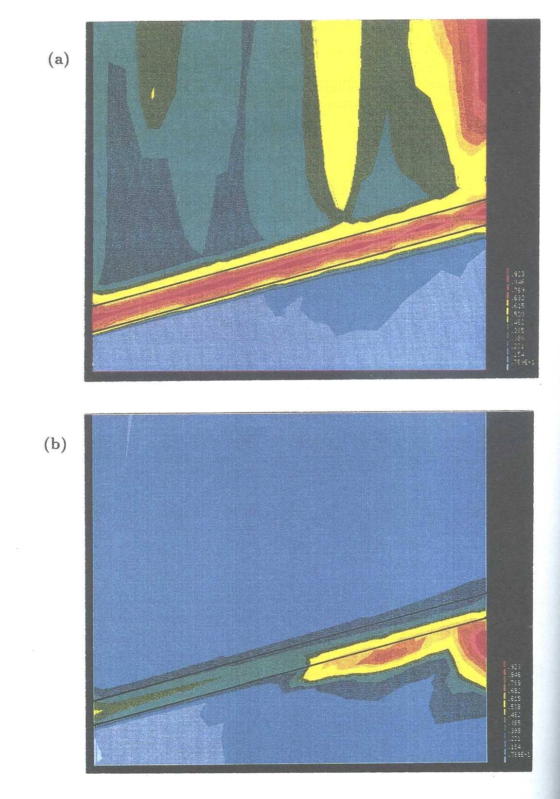
The modified eight derivative multiple isomorphous map of Bacillus subtilis pectate lyase revealed a new protein architecture; the right handed parallel B-coil. The Cray YMP has been used to build and refine this structure using the program XPLOR (A.T. Brunger, X-PLOR manual - version 2.1, (Yale University, New Haven, CT, 1990)]. Structural information was used to improve the quality of the phases in an iterative procedure. XPLOR improves the efficiency of refinement and map interpretation since it escapes the problem of the limited radius of convergence of least squares methods by using molecular dynamics. The X-ray restraints are applied as a term in the equation used to evaluate the energy of the system (X-ray restraints are the observed structure factor amplitude possibly weighted by the experimental phase). At the time of writing (early July 1993) the figure of merit (the cosine of the phase error) has improved from 0.53 for 8439 reflections to 3.0Å to 0. 70 for 13724 reflections at 2.5Å. Refinement is continuing and is expected to be complete at 2.35Å by the time this summary appears. The structure will then be refined at 1.9Å.
The β-coil structure is strikingly regular and allows the favourable stacking of aromatic residues shown in the Figure 1 below. The 399 residue pectate lyase structure consists of eight turns of β-coil with loops that form a second domain. The active site is between these domains as identified by the calcium binding site that is essential for the specificity of pectate lyase as opposed to pectin lyase.
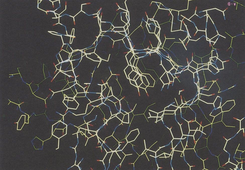
The majority of proteins are glycosylated, i.e. they have attached oligosaccharide chains which can have various effects on conformation, function, antigenicity and dynamics. There are several attributes of these oligosaccharides that make analysis difficult by conventional techniques, but their relevance to many glycoprotein structure/function relationships means they can no longer be ignored. Computer graphics has found a particular niche in their conformational studies, backed up with NMR data, and where possible, X-ray crystallography. Both the physicochemical techniques have the limitation of being unable to view the dynamics of these often flexible, heterogeneous moieties: NMR because the molecular timescale is too slow and results can only reflect a conformationally averaged ensemble of structures; X-ray crystallography because crystals for high resolution studies are not forthcoming, and any novel strategies adopted for crystallisation will lead to artificial solutions.
We are using computer graphics in three main areas:
For the first, access to the CRAY is important to study empirical quantum mechanical solutions in the presence of water to define the orientation of functional groups for interaction with specific protein motifs. In the second approach, the cpu of a CRAY is essential for molecular dynamic studies of molecules above the 10,000 molecular weight range which are inaccessible to NMR studes. Thirdly, we are carrying out a series of molecular mechanical studies of the interactions of MHC from which we can predict activities in in vitro cell assays; hence there is a large cpu need to produce a statistically valid data set. [MHC = Major histocompatibility antigen-protein domains of molecular weight around l0kD]
We are networked through to the CRAY via a Silicon Graphics workstation, running Biosym software. Comparisons are drawn between conformational studies using different force fields ( CVFF and AMBER) with different oligosaccharide parameters, dielectric constants, and simulated water environments.
1. Molecular modeling of 27kD of gp/120, the envelope glycoprotein the HIV virus. This is a highly glycosylated molecule for which X-ray crystallography in its native glycosylated state is not possible. The studies have shown the dynamics of the oligosaccharide chains in relationship to the protein and highlighted areas accessible for protein-protein interactions important in AIDS pathogenesis. We predict that the accessible areas will be processed for interaction with MHC and have used the CRAY to study the relative affinities of MHC interactions with various peptides. This is important in understanding of tolerance in the immune system. The sequelae of the studies are also important in other autoimmune diseases and infectious pathologies.
2. Carrying on from studies on the Silicon Graphics we are defining ways to accurately visualise oligosaccharide conformation. We have used the CRAY to look at anionic oligosaccharides in water and predict their interactions with proteins important in novel drug design in strategies in AIDS, inflammation and cancer. We are also using de nova approaches to study fully relaxed maps of mono-to-oligosaccharides and molecular orbital and charge effects. The ability to use the Biosym software run on the CRAY for these tasks has enabled us to carry out novel parameterisation of forcefields specific for oligosaccharide modeling and extensive molecular dynamics.
Hounsell, E.F., Davies, M.J. and Renouf, D.V. (1992) Studies of oligosaccharide and glycoprotein conformation. Biochem. Soc. Trans.;20:259-264.
Hounsell, E.F. Conformational studies of glycoproteins. (1992) 6th International Polysaccharide Symposium.
Hounsell, E.F. and Renouf, D.V. (1992) Glycoprotein and oligosaccharide conformation studies in Band T cell immunology. Italian Biochemistry and Chemistry Societies Joint Symposium.
Renouf, D.V. and Hounsell, E.F. (1992) Exploration of the conformational space sampled by N-acetyllactosamine sequences and their derivatives having Fuca, GalNaca, GlcNaca and NeuAca substituents. Second Symposium on Oligosaccharide Conformation, Nantes, 1992.
Hounsell, E.F. (1992) Epitope modelling in glycoimmunology. Second Jenner, International Glycoimmunology Meeting In: Annals Rheum.Dis.; November:1270-1271.
Renouf, D.V. and Hounsell, E.F. {1993) Conformational studies of the backbone (poly-N-acetyllactosamine) and the core region sequencesof O-linked carbohydrate chains. Int.J.Biol.Macromol.; 15:37-42.
Hounsell, E.F.and Davies, M.J. (1993) Role of protein glycosylation in immune regulation. Annals Rheum. Dis.;52:S22-S29.
Renouf, D.V. and Hounsell, E.F. (1993) Molecular dynamic studies of O-linked core 1 protein glycosylation sequences. Royal Society of Chemistry Carbohydrate Group, Dundee April 1993.
Hounsell, E.F. (1993) Structural and conformational studies of glycoproteins and oligosaccharide recognition determinants. NATO Workshop on NMR of Biological Macromolecules.
Hounsell, E.F. (1993) Royal Institution Lecture. Drug design based on oligosaccharide-to-protein interactions.
Monte Carlo track structure simulation has become an important tool in biophysical modelling of radiation effects in mammalian cells. The criticial importance of clustered properties of radiation tracks in determining their biological properties cannot be measured over dimensions of less than tens of nm by current experimental methods. The availability of Monte Carlo track structure codes which simulate radiation tracks, molecular interaction by interaction of all ionizations and excitations (in the very early physical stage (0-10-15 s) and in the pre-chemical stage (10-15 - 10-12 s)), has in more recent years made it possible to make theoretical investigation of those clustered properties down to dimensions, less than 1 nm. In this report a brief description is given for Monte Carlo track structure Codes which have been developed for the transport of electrons and ions in water. Monte Carlo track structure methods and supercomputers have made it possible to perform calculations in a region where experimental data are impossible to obtain and analytical methods are not applicable.
The Code kurbuc (1) is the first code which simulates tracks of energetic electrons in water vapour in the energy range of 10 eV to 10 MeV. Total elastic, ionization and excitation cross sections compiled for the code are given in Fig. (1). The elastic cross sections were obtained from Rutherford's formula taking into account the screening parameter η. The differential cross section (dσ/dΩ) is given by:
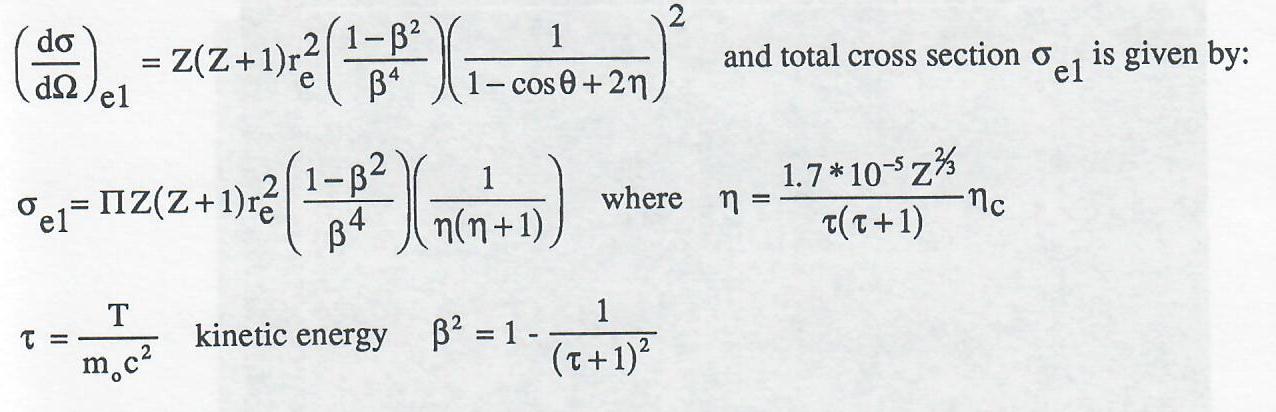
As Rutherford's formula is inadequate in describing elastic scattering at low energies various experimental data were used to obtain cross sections below 1 keV.
The ionization cross sections above 10 keV were calculated according to Weizacker-Williams method. The differential cross section is given as the sum of close and distant collisions.
where the first term, describes the collision between two electrons and the second term, describes the interaction of the equivalent radiation field with the orbital electrons. The ionization cross sections below 10keV were compiled from various sources.
The total excitation cross sections were derived from the method given by Berger and Wang(2) and Paretzke (3). Full detailed description of this Code is given elsewhere (1).
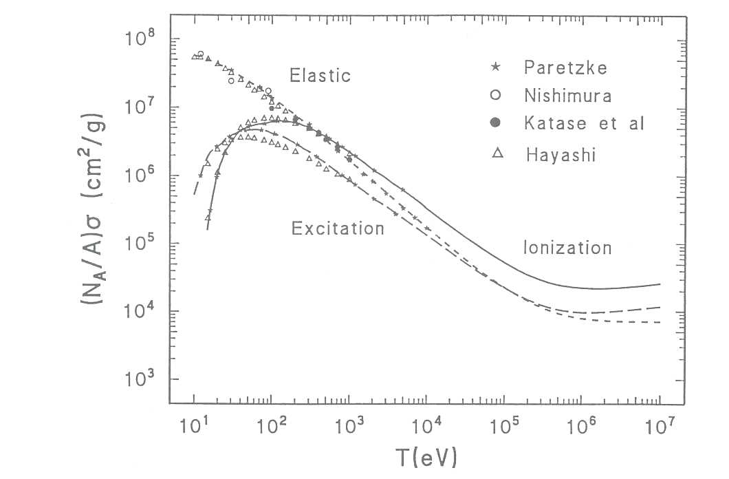
Space and time evolution of chemical species produced following the initial physical stage of interaction of ionizing particle with the medium has been obtained with the code CPA100 (5). Fig (2) gives distribution of initial ionization and excitations at 10-15s, hydroxyle radicals (OH) and hydrated electrons at 10-12 s, following the physico-chemical step (10-15 10-12 s), for a 1 keV electron set in motion in liquid water. The physical and chemical tracks have been used to investigate mechanism of radiation damage in biological molecules.
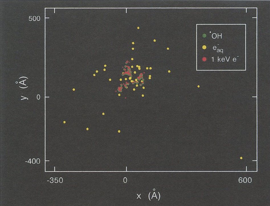
PITS (6) (Positive Ion Track Structure) is a code written for simulating positive ion tracks in a variety of media, with and without secondary electron transport. The basic concept is schematically described in Fig. (3).
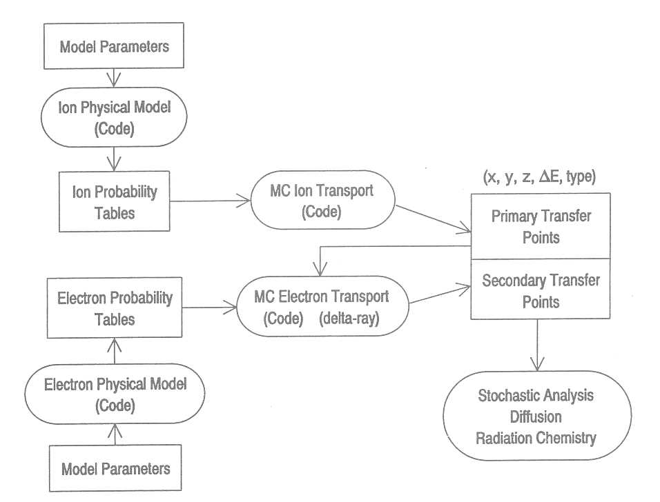
The Code has been interfaced with several module for the transport of the secondary electrons (delta-rays) for water and water vapour C4). Fig. (4) shows a segment of a 1 MeV proton generated in water vapour. The data shows ionizations and excitations produced by the primary particle (proton) and the secondary electrons (delta electrons).
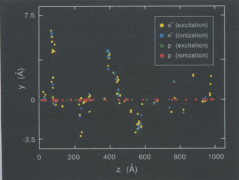
An understanding of the mechanisms of damage in biological targets by ionizing radiation requires a knowledge of spatial distribution of energy loss in subcellular structures such as DNA and higher order structures. The conceptual framework is to irradiate the volume of interest (such as DNA) by the given radiation field and then obtain the energy deposited in the target volume by comparing the position of all ionizations and excitations with the volume occupied by the target. Fig. (5) shows the distributions for a target similar to a linear segment of DNA. The left ordinate shows comparison of distributions of absolute frequency of energy depositions in a cylindrical volume of dimensions similar to a segment of DNA randomly positioned and oriented in water and irradiated with 1 Gy of the given radiation.
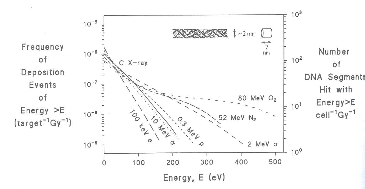
These calculations provide data on absolute frequencies of energy deposition events in different target size volume from which other microdosimetric quantities can be calculated.
1. Uehara, S., Nikjoo, H., and Goodhead, D.T. 1993. Cross-sections for water vapour for Monte Carlo electron track structure code from 10 eV to 10 MeV region. Physics in Medicine and Biology (in press).
2. Berger, M.J. and Wang, R. 1988. Multiple scattering angular deflections and energy-loss straggling. In: Monte Carlo Transport of Electrons and Photons. eds. T.M. Jenkins W.R.Nelson and A. Rindi (Plenum Press, New York) pp. 21-56.
3. Paretzke, H.G. 1987. Radiation track structure theory. In: Kinetics of non-homogeneous Processes, ed. G.R. Freeman (Wiley-Interscience, New York) pp. 89-170.
4. Nikjoo, H. and Uehara, S. 1993. Comparison of various Monte Carlo Track Structure Codes for energetic electrons in gaseous and liquid water. In: Proceedings of DOE Workshop on Computational approaches in Molecular Radiation Biology: Monte Carlo Methods. eds M.N. Varma, A. Chatterjee, April 1993, Irvine (in press).
5. Terrissol, M. and Beaudre, A. 1990. Simulations of space and time evolutions of radiolytic species induced by electrons in water. Radiation Protection Dosimetry, .31, pp. 175-178.
6. Wilson, W.E., Miller, J.H. and Nikjoo, H. PITS: A code set for Positive Ion Track Structure. In: Proceedings of DOE Workshop on Computational approaches in Molecular Radiation Biology: Monte Carlo Methods. eds. M.N. Varma, A. Chatterjee, April 1993, Irviine (in press).
1. Uehara, S., Nikjoo, H., and Goodhead, D.T. 1993. Cross-sections for water vapour for Monte Carlo electron track structure code from 10 eV to 10 MeV region. Physics in Medicine and Biology (in press).
2. Nikjoo, H. and Uehara, S. 1993. Comparison of various Monte Carlo Track Structure Codes for energetic electrons in gaseous and liquid water. In: Proceedings of DOE Workshop on Computational approaches in Molecular Radiation Biology: Monte Carlo Methods. eds. M.N. Varma, A. Chatterjee, April 1993, Irvine (in press).
3. Wilson, W.E., Miller, J.H. and Nikjoo, H. PITS: A code set for Positive Ion Track Structure. In: Proceedings of DOE Workshop on Computational approaches in Molecular Radiation Biology: Monte Carlo Methods. eds. M.N. Varma, A. Chatterjee, April 1993, Irvine (in press).
4. Nikjoo H, Charlton, D.E, Goodhead D.T, 1993. Monte Carlo track structure studies of energy deposition and calculation of initial dsb and RBE. In: Mechanisms Underlying Cellular Radiosensitivity and RBE, Ed. Ann B. Cox. Advances in Space Research, Pergamon Press. (in press)
5. Charlton D.E. and Nikjoo H., 1992. An attempt to model the increase of radiation sensitivity due to the incorporation of cold IUdR or BrdU into DNA of irradiated cells. In: Biophysical Aspects of Auger Processes, Eds. R.W. Howell, V.R. Narra, K.S.R. Sastry, D.V. Rao. AAPM, pp 51-65.
6. Nikjoo H., Savage J.R.K., Charlton D.E., Harvey A., 1992. Test of radiation damage enhancement due to incorporation of BrdU into DNA using chromatid abberations. In: Biophysical Aspects of Auger Processes, Eds. R.W. Howell, V.R. Narra, K.S.R. Sastry, D.V. Rao. AAPM, pp 66-79.
7. Charlton D.E., Nikjoo H., Goodhead D.T. 1992. Calculation of Energy depositions in nanometer volumes using track structure methods: Comparison with other approaches. In Radiation Research, "A Twentieth-Century Perspective", Eds. Chapman, Dewey, Whitmore. Vol II. Academic Press. Academinc Press, pp 421-426
8. Nikjoo H., Harvey A, Savage J.R.K., Charlton D.E., 1991. A test of theoretical radio-sensitzation radiation of BrdU incorporation using chromatid aberration. In: Radiation Research, "A Twentieth-Century Perspective", Eds. Chapman, Dewey, Whitmore. Vol I. Academinc Press, p 414
9. Nikjoo H., Harvey A., Savage J.R.K, Charlton,D., 1991. Monte Carlo track Structure Calculations of Cellular DNA Damage. lnt. J. Radiat. Biol., vol 60, 6, 932. [abstract]
10. H. Nikjoo, D.T. Goodhead, D.E. Charlton and H.G. Paretzke, 1991. Energy deposition in cylindrical volume by monoenergetic elctrons 10 eV - 100 keV. lnt. J. Radiat. Biol. vol 60, 5, pp 739-756
In recent years, point mutations in Factor IX have been recorded in a database which has been made available to the international academic community. All of these mutations, which have been detected from DNA sequencing, cause a blood clotting deficiency which leads to the haemorrhagic disorder haemophilia (B Christmas disease).
Factor IX is a multi-domain protein. The key domains are as follows:
In the clotting cascade another coagulation protein, Factor XIa converts Factor IX into its active form which is known as Factor IXa. This, in turn, catalyses the formation of Factor Xa in the next stage of the clotting process - which leads, eventually, to the conversion of fibrinogen to fibrin by thrombin.
Factor IX is known to bind calcium ions and has a cofactor, Factor VIIIa which is essential for function. Many of the molecular details of the clotting cascade remain unclear, and the current study has the aim of investigating functional regions of Factor IX.
The mutations in Factor IX fall into two groups depending on the level of antigen activity compared to clotting activity. Where both are low, the mutant is said to be cross-reacting material negative ( crm-). If, however, there is significant antigenic activity, the mutation is classified as cross-reacting material positive ( crm+). We have confined our study to crm+ mutants, as these molecules have defects in functional regions which lead to loss of biological activity.
We have built and refined models of the G1a domain and the serine protease domain using standard methods. The Cray was used for some of this work. We then performed residue replacements for all the crm+ mutants in the database.
Many of the mutations lead to severe van der Waals interactions between the mutated residue and neighbouring residues. In such cases, we have been able to use the Cray to perform fast minimisations on such mutant molecules. Study of these mutants shows how relaxation of the protein into a more energetically favourable conformation often distorts regions of the protein involved in calcium and substrate binding. We have also been able to identify surface residues which may be involved in cofactor binding and this has suggested relevant experiments for further investigation.
There is increasing evidence that oligonucleotide sequences may adopt curved conformations either because of sequence directed, intrinsic, bending or on iteraction with proteins. Thus, the axis through the double helix is no longer straight. Such curvature of the helix effects recognition properties by changing such structural features such as groove width. The structural data on oligonucleotide sequences are based mainly on those whose structures have been crystallised and these tend to be fairly short (i.e. around 12 base-pairs) with only a small amount of curvature. Gel retardation experiments have provided most of the data on intrinsic bending (but not 30 models) and in contrast they tend to be on much longer sequences, typically 50 base-pairs or longer. Moreover, they often contain sequence repeats in line with the known helical repeat of B-DNA which increase the amount of curvature. The advent of more powerful supercomputers has allowed us to bridge this gap in sequence length as we have now generated 30 atomic level models of 51 base-pair DNA in solution.
These models have been generated with the AMBER 4.0 package using the molecular dynamics models. Typical calculations contain around 2400 atoms and we have used a distance dependent dielectric constant together with hydrated counter-ions to model the surrounding aqueous solution. Simulations are carried out at constant number of atoms and constant volume with the system connected to a heat bath at 298K. So far, we have simulated 500 ps of dynamics using a time-step of 2 fs.
We are just beginning to examine these results in detail. We have generated a 'movie' on our own Silicon Graphics Indigo in order to visualise the change in conformation during the simulation. We can clearly see large changes in the overall curvature of the structure as it moves away from from the initial straight helix towards a 'skipping rope' conformation. This can be seen clearly by comparing the initial conformation (Figure 1) and the average conformation over the last 200 ps (Figure 2).
We have colour coded different parts of the sequence such that the regions in which there are adenine-thymine base pairs (A-tract) are yellow. The centre of curvature appears to be approximately at the mid-point of the sequence as expected from experimental gel retardation experiments. We estimate that the radius of curvature is around 0. The local hydrogen bond conformation are very constant over 500 ps with nearly all the Watson-Crick hydrogen bonds being maintained through out the simulation. Occasionally breaking and reforming of hydrogen bonds occurs but overall they are very stable. Further analysis of the curved conformation is continuing with the aim of relating curvature to local sequence.
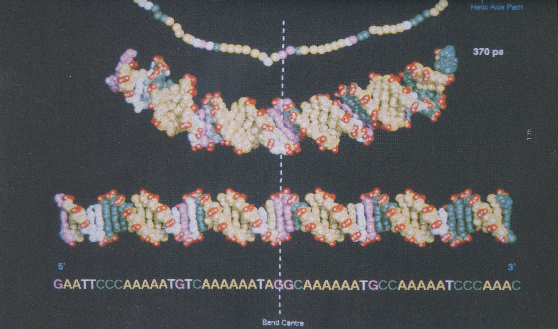
The work of the group over the past two years can be considered under four sub-headings; one concerned with applications of a particular technique (free energy perturbation), and three distinct macromolecular topics.
The importance of computing free energies rather than enthalpies can scarcely be overstressed. Experimental measurements almost invariably involve free energies in the form of equilibrium constants of one sort or another and the influence of solvent is crucial. The technique is becoming a standard method and was reviewed by us [1] and also put on a firmer footing with respect to the atom-based charges used in simulations. [2,3] Applications include the computation of electrode potentials [4] as a prerequisite for the design of bioreductive anti-cancer drugs; partition functions which relate to drug transport [5] tautomer ratios which have relevance to the binding of folate to dihydrofolate reductase [6] and solvation energies. [7]
No computations of biological properties are really acceptable without the incorporation of solvent, ideally with explicit water molecules. Such simulations are massive and need the power of the CRAY supercomputers.
Protein structure prediction starts by using similarities between the sequence of the protein of interest and one of known structure from the database of X-ray crystals coordinates. There then follows graphical modelling, but the final stage is the energy minimization of the solvated structure and molecular dynamics to shake the predicted structure into its minimum conformation. It is this final crucial step which employs supercomputers.
During the grant period this outline has been followed [8] for beta-factor XIIa and most outstandingly with inteleukin-4 and its receptor. [9] This latter work is the high spot of the research during the grant period and was featured both on Channel 4 news in the UK and internationally by CNN.
The structure of the cytokine interleukin 4 was predicted independently of nmr evidence and found to be in good agreement. It is a small protein, within the limited scope of nmr and significant as a messenger in the immune system. Far more important is its receptor (the IL-4 receptor) which is membrane-bound and thus essentially beyond the capabilities of X-ray crystallography or nmr.
We modelled the receptor structure based on the crystal structure of CD4 Refinement by molecular dynamics leads to a suggested structure which has been docked to interleukin 4, identifying several residues of importance for binding. This is the starting point for the development of drugs to prevent the immune message being passed: drugs which could have a role in the treatment of asthma.
The colour plate shows the small IL-4 cytokine messenger protein (in blue), binding to our model of the dimeric IL-4 receptor.
In our search for sequence-specific ligands which bind to DNA we have focussed on the fascinating small polyanion, spermine. The biological function of this message carrier is not fully clear but it does control DNA conformation and may play a role in deciding which sections of DNA are read. It can change right-handed DNA helices into left-handed in the test tube. Supercomputer power has enabled us to simulate at least the opening stage of this transformation. [10]
The power and memory available at the Atlas Centre has permitted us to start what is our most ambitious biomolecular study yet and one with long-term importance. We have built a model of a biological bilayer membrane (DMPC) complete with a ten Angstrom layer of water each side; phosphatidylcholine head-groups and even solutes. The simulated membrane is in accord with all available data from nmr and neutron scattering. It is our intention to insert cholesterol and even protein into this model and to study drug transport and partition. [5]
1. C.A. Reynolds, P.M. King and W.G. Richards, Free energy calculations in molecular biophysics, Mol. Phys. 76 (1992) 251
2. C.A. Reynolds, J.W. Essex and W.G. Richards, Atomic charges for variable molecular conformations J. Am. Chem. Soc. 114 (1992) 9075
3. C.A. Reynolds, J.W. Essex and W.G. Richards, Errors in free-energy perturbation calculations due to neglecting the conformational variation of atomic charges, Chem. Phys. Lett. 199 (1992) 257
4. S.G. Lister, C.A. Reynolds and W.G. Richards, Theoretical calculation of electrode potentials: electron withdrawing compounds, Int. J. Quantum. Chem. 41 (1992) 293
5. J.W. Essex, C.A. Reynolds and W.G. Richards, Theoretical determination of partition coefficients, J. Am. Chem. Soc. 114 (1992) 3634
6. C.H. Schwalbe, D.R. Lowis and W.G. Richards, Pterin 1H-3H tautomerism and its possible relevance to the binding of folate to dihydrofolate reductase, J. Chem. Soc. Chem. Commun. 1199 (1993)
7. A.H. Elcock and W.G. Richards, Relative hydration free energies of nucleic acid bases, J. Am. Chem. Soc. 115 (1993) 7930
8. M.J. Ramos and W.G. Richards Computer models of beta-factor XIIa and inhibitor, Drug News and Perspectives 5 (1992) 325
9. P. Bamborough, G.H. Grant, C.J.R. Hedgecock, S.P. West and W.G. Richards, A computer model of the interleukin-4 receptor complex PROTEINS, Structure, Function and Genetics 17 (1993) 11
10. LS. Haworth, A. Rodger and W.G. Richards, A molecular dynamics simulation of a polyamine-induced conformational change of DNA. A possible mechanism for the B to Z transition, J. Biomolec. Struc. Dynam. 10 (1992) 195
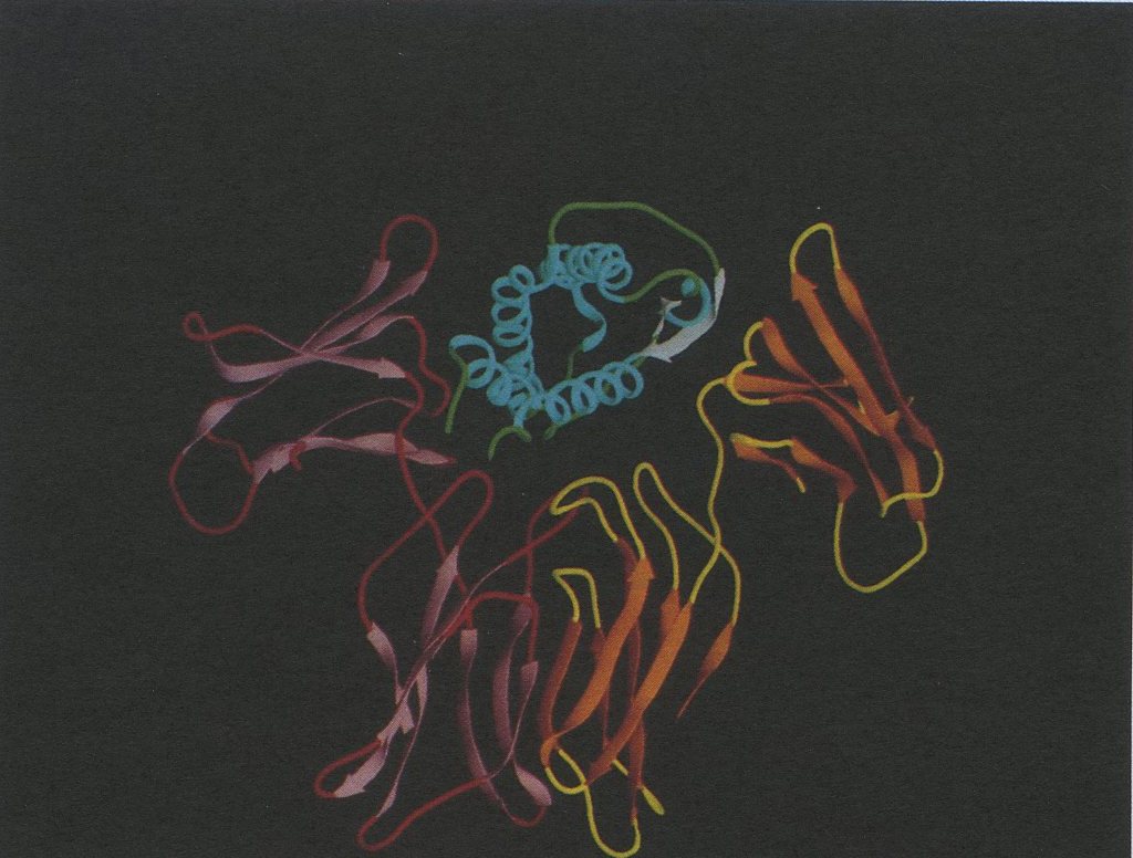
C.A. Reynolds, P.M. King and W.G. Richards Free energy calculations in molecular biophysics Mol. Phys. 76 (1992) 251
C.A. Reynolds, J.W. Essex and W.G. Richards Atomic charges for variable molecular conformations J. Am. Chem. Soc. 114 (1992) 9075
C.A. Reynolds, J.W. Essex and W.G. Richards Errors in free-energy perturbation calculations due to neglecting the conformational variation of atomic charges Chem. Phys. Lett. 199 (1992) 257 -
S.G. Lister, C.A. Reynolds and W.G. Richards Theoretical calculation of electrode potentials: electron withdrawing compounds lnt. J. Quantum. Chem. 41 (1992) 293
J.W. Essex, C.A. Reynolds and W.G. Richards Theoretical determination of partition coefficients J. Am. Chem. Soc. 114 (1992) 3634
C.H. Schwalbe, D.R. Lowis and W.G. Richards Pterin 1 H-3H tautomerism and its possible relevance to the binding of folate to dihydrofolate reductase J. Chem. Soc. Chem. Commun. 1199 (1993)
A.H. Elcock and W.G. Richards Relative hydration free energies of nucleic acid bases J. Am. Chem. Soc. 115 (1993) 7930
M.J. Ramos and W.G. Richards Computer models of beta-factor XIIa and inhibitor Drug News and Perspectives 5 (1992) 325
P. Bamborough, G.H. Grant, C.J.R. Hedgecock, S.P. West and W.G. Richards A computer model of the interleukin-4 receptor complex PROTEINS, Structure, Function and Genetics 17 (1993) 11
LS. Haworth, A. Rodger and W.G. Richards A molecular dynamics simulation of a polyamine-induced conformational change of DNA. A possible mechanism for the B to Z transition J. Biomolec. Struc. Dynam. 10 (1992) 195
This grant of 1200 hours at RAL and 800 hours at ULCC was used to further our research in quantum chemistry and theoretical spectroscopy. As outlined in the proposal, and described in detail as attached, we have worked on (a) Coupled Cluster Theory, in particular Brueckner Theory (b) Higher derivatives of the potential energy surface. A quartic force field and related spectroscopic constants have been calculated for benzene (c) The variational method for rovibrational energies has been used to calculate high accuracy potential surfaces for CH2, C2H2, NH2 and HCN (d) Collaborations with colleagues on problems in organic chemistry (e) Development of the Restricted Open Shell Moller-Plesset method (f) Development of a new Density Functional Code (g) Continuing development of our software package CADPAC
As stated in the application, this WAS our major computer time facility for the two years 1991-1993. All our computer time requested and awarded (1200 hours RAL, 800 hours ULCC) was used. Much development work was possible on our own (SERC partially funded) Convex C220 but no computer code is worthwhile in quantum chemistry and theoretical spectroscopy unless it becomes a production code and hence our need for and use of national facilities. We have continued to develop our in-house quantum chemistry package CADPAC (now version 5.1). In this period new features were added, in particular our Brueckner Coupled Cluster code. Much work was done on speeding up the integral evaluation. The higher derivatives code was made more robust. More recently Density Functional Theory has been added (but it does not properly form part of this report). We outline below scientific advances we have made which benefited by the availability of the national resources. A list of Published papers is given at the end.
In quantum chemistry we have continued to develop test and use the most sophisticated Methods. In particular R Kobayashi and RDA have continued examining the coupled cluster method looking at its most elegant form using Brueckner orbitals for which the wavefunction is exp(T2)χ. Gradient theory has been developed for this BD theory [169] and the inclusion of the effects of triple replacements BD(T) [175]. A comparison of this Brueckner variant with the standard CCSD (using SCF orbitals) has been published [182], in which it is argued that the effect of triple replacements is more important than the differences between the methods. The greatest difference arises in i.r. intensities, but it is difficult to tell which is the most reliable method. Large basis set studies suggest that BD(T) harmonic frequencies are within 10 cm-1 of experiment. We have looked at electron densities as represented by Brueckner orbitals and shown that they are close to MCSCF densities [194]. We have used the BD(T) method to perform definitive structure and frequency calculations on Si2H4. We have looked at the importance of using large basis sets within the BD(T) approach [213]. In summary we have used computer time to develop, test and use the BD(T) ab initio method for electron correlation, with the result that we have a highly efficient and high accuracy code. To our knowledge it is the only such Brueckner specific code, in general use, in existence.
We have continued to develop and use advanced gradient theory for the determination of spectroscopic properties. At the Self Consistent Field (SCF) level, our programs for the calculation of analytic third [153] and fourth [174] energy derivatives, and higher dipole derivatives [179] are in production. One very important application has been the determination of the quartic force field of benzene [139], long awaited by the spectroscopists. A complete set of anharmonic constants was presented; it may never be possible for the experimentalist to calculate reliably off-diagonal xij. Our values will be benchmarks for years to come we also presented an i.r. spectrum, up to 4000 cm-1, with several new assignments of experimental bands. We believe that these calculations fill many gaps in the understanding of the spectroscopy of benzene. The force fields so derived ab initio are analysed using SPECTRO [150]. Other molecules studied using derivative theory include CH2F2 [163]. Higher accuracy quartic force fields were determined using the MP2 method, by finite difference procedures. The use of such force fields was demonstrated by explaining the 2v8, v1 and v6 experimental bands and intensities by assigning v1 and v6 as (v1, v4+v8+v2) and (v6, 2v2) doublets. We are currently performing a similar analysis of CH2Cl2. We have also studied FSN [211], a difficult molecule for which excellent predictions were obtained by scaling the quadratic and cubic force constants of a CASSCF force field.
We have continued to develop and use our variational method for the high accuracy study of rovibrational properties of three and four atom molecules. In particular we have studied the Renner-Teller pair of surfaces (1A1, 1B1) of CH2 to assign observed vibronic bands (162], finding that many of the previous band labels were incorrect. Collaborative work with P Rosmus has been reported on the 2B1 - 2A1 spectrum of BH2 [183], the 2A2-2B1 spectrum of H2O+ (205] and band intensities of water vapour (208]. Our most significant study to date is that of the 2B1 , 2A1 surfaces of NH2 [221] where we determined rovibrational levels (J≤9/2) to 20,000 cm-1, for which the agreement with all known levels is to within a few cm-1. With I. Mills, we have used this approach to obtain a high accuracy force field of HCN (207] and to obtain a good equilibrium structure of this molecule (184]. This successful work has been extended to four atoms with preliminary calculations on H2S2 [167] and CHNO [191]. We have refined a force field for C2H2 [192]. It should be realised that these variational calculations are very time consuming because the non-linear optimisation of force field parameters to observed rovibrational transitions is at present a trial and error non systematic procedure. Even so, we believe that this is the only reliable way to obtain the highest accuracy force fields (as for NH2 above).
We have collaborated with colleagues on problems in organic chemistry. With A J Kirby we have studied ab initio the gauche effect on bond length and reactivity [170] by examining Y-CH2-CH2-OX, looking at the effects of > β-substituents on C-OX bonds. With S A Vasquez, we have studied the three oxidation forms of lumiflavin [177]. We have collaborated with S L Price to study the electrostatic interaction of peptides [226].
We have used extra available time (principally at ULCC) for the following studies:
For the last 18 months we have been developing our approach for Density Functional Theory. We have published a number of papers [187, 195, 198, 200, 201, 202, 204, 209, 212, 213, 214, 216, 220] which have required use of both our own and national facilities. We think that it is probably best to give a full report of our DFT nvestigations on the next occasion, and so we confine ourselves to the comment that DFT, on our evidence (and of course that of others), appears to be a very important tool for computational chemistry. Structures and energetics, especially for larger molecules, are considerably more reliably predicted than at the SCF level of theory.
The proposal suggested that we Might work on anharmonic potential surfaces, on Brueckner theory y, on the variational method for rovibational energy levels (specifically NH2). All of these we have studied in depth as reported above. Other topics were suggested, such as spin-projected UHF MP2, which has become Restricted Open Shell MP and is now the accepted way for this problem. And of course we have moved into Density Functional Theory.
150. SPECTRO - a program for the derivation of spectroscopic constants from provided quartic force fields and cubic dipole fields. J F Gaw, A Willetts, W H Green and N C Handy, Advances in Molecular Vibrations and Collision Dynamics. ed. J M Bowman, JAI, Greenwich CT, IB,169 185 (1991).
153. Higher Analytic Derivatives. (1) A new implementation for the third derivative of the SCF energy. S M Colwell, D Jayatilaka, P E Maslen, R D Amos and N C Handy. Int J Quant Chem. Q 179 (1991).
160. Transition states from Molecular Symmetry Groups: Analysis of NonRigid Acetylene Trimer. R G A Bone, T W Rowlands, N C Handy and A J Stone. Molec. Phys, Z2, 33 (1991).
162. Theoretical Assignment of the Visible Spectrum of Singlet Methylene.
W H Green, N C Handy, P J Knowles and S Carter. J Chem Phys 94, 118 (1991).
164. Some investigations of the MP2-R12 method. M.J. Bearpark, N .C. Handy, R.D. Amos and P.E. Maslen. Theor Chim Acta. 79, 361 (1991).
165. The calculation of Frequency Dependent Polarizabilities as PseudoEnergy Derivatives. J.E. Rice and N .C. Handy. J. Chem. Phys. 94, 4959 (1991)
166. Vibration-rotation coordinates and kinetic energy operators for polyatomic molecules M.J. Bramley, W.H. Green and N.C. Handy. Molec. Phys. 73, 1183 (1991)
167. A study of the ground electronic state of disulphane. M-D Su, A. Willetts, M.J. Bramley and N.C. Handy. Molec. Phys. 73, 1209 (1991)
168. An harmonic Vibrational Properties of CH2F2: A comparison of theory and experiment. R.D. Amos, N.C. Handy, W.H. Green, D. Jayatilaka, A. Willetts and P. Palmieri. J .Chem. Phys. 95, 8323 (1991)
169. Gradient Theory Applied to the Brueckner Doubles Method. R. Kobayashi, N.C. Handy, R.D. Amos, G.W. Trucks, M.J. Frisch and J.A. Pople. J. Chem. Phys. 95, 6723 (1991)
170. Bond Length and Reactivity: the Gauche Effect. A combined Crystallographic and Theoretical Investigation of the Effects of b-substituents on C-OX Bond Length. R.D. Amos, N .C. Handy, P.G. Jones, A.J .Kirby, J .K. Parker, J.M. Percy and M-D Su. J. Chem. Soc. Perkin Trans. 2, 549 (1992)
171. Implications of Unitary Invariance for Gradient Theory. D.Jayatilaka and N.C. Handy. Int. J. Quantum Chem. 42, 445 (1992)
172. Spin Contamination in Single-Determinant Wave functions. J .S. Andrews, D. Jayatilaka, R.G.A. Bone, N.C.Handy and R.D.Amos. Chem. Phys. Lett. 183. 423 (1991)
173. The Calculation of Frequency Dependent Hyperpolarizabilities including Electron Correlation Effects. J. E. Rice and N. C. Handy. Int. J. Quantum Chem. 43, 91 (1992)
174. Higher Analytic Derivatives. (2) The Fourth Derivative of the Self Consistent Field Energy. P. E. Maslen, D. Jayatilaka, S. M. Colwell, R. D. Amos and N. C. Handy. J. Chem. Phys. 95, 7409 (1991)
175. The Analytic Gradient of the Perturbative Triple Excitations Correction to the Brueckner Doubles Method. R. Kobayashi, R. D. Amos and N. C. Handy. Chem. Phys. Lett. 184, 195 (1991)
176. Open Shell Moller-Plesset Perturbation Theory. R. D. Amos, J. S. Andrews, N. C. Handy and P. J. Knowles. Chem. Phys. Lett. 185, 256 (1991)
177. An Investigation of the Three Oxidation Forms of Lumiflavin. S. A. Vazquez, J. S. Andrews, C.W. Murray, R. D. Amos and N. C. Handy. J. Chem. Soc. Perkin Trans. 2, 889 (1992)
178. Restricted Moller-Plesset Theory for Open Shell Molecules. P. J. Knowles, J. S. Andrews, R. D. Amos, N. C. Handy and J. A. Pople. Chem. Phys. Lett. 186, 130 (1991)
179. Higher Analytic Derivatives (3) Geometrical Derivatives of the Dipole and Dipole Polaris abilities. D. Jayatilaka, P. E. Maslen, R. D. Amos, and N. C. Handy. Molec. Phys. 75, 271 (1992)
180. On the Optimisation of Exponents for d and f Polarisation Functions for First Row Atoms. M. J. Bear park and N. C. Handy. The or. Chim. Act a - , 115 (1992)
181. Cumulative Reaction Probabilities for H+H2 → H2+H from a knowledge of the Anharmonic Force Field. M. J. Cohen, N. C. Handy, R. Hernandez and W. H .Miller. Chem. Phys. Lett. 192, 407 (1992)
182. Comparison of the Brueckner and Coupled-Cluster Approaches to Electron Correlation. T. J. Lee, R. Kobayashi, N. C. Handy and R. D. Amos. J. Chem. Phys. 96 8931 (1992)
183. Rovibronic 2B1 (θu) - 2A1 Spectrum of the BH2 Radical. M. Brommer, P. Rosmus, S. Carter and N. C. Handy. Molec. Phys. 77 549 (1992)
184. The Equilbrium Structure of HCN. S. Carter, I. M. Mills and N. C. Handy. J. Chem. Phys. 97, 1606 (1992)
185. Theoretical Calculations of the Nuclear Magnetic Shielding Tensors for the Ethylenic Carbon Atoms in Cyclopropenes. C. M. Smith, R. D. Amos and N. C. Handy. Molec. Phys. 77 381 (1992) 186. Higher Analytic Derivatives IV. An harmonic Effects in the Benzene Spectrum. P. E. Maslen, N. C. Handy, R. D. Amos and D. Jayatilaka. J. Chem. Phys. 97, 4233 (1992)
187. Quadrature Schemes for Integrals of Density Functional Theory. C. W. Murray, N. C. Handy and G. J. Laming. Molec. Phys. 78, 997 (1993)
188. Comparison and Assessment of Different Forms of Open Shell Perturbation Theory. C. W. Murray and N. C. Handy. J. Chem. Phys. 97, 6509 (1992)
189. The Harmonic Frequencies of Benzene. N. C. Handy, P. E. Maslen, R. D. Amos, J. S. Andrews, C. W. Murray and G. J. Laming. Chem. Phys. Lett. 197, 506 (1992)
190. Efficient Calculation of Rovibrational Eigenstates of Sequentially-Bonded Four-Atom Molecules. M. J. Bramley and N. C. Handy. J. Chem. Phys. 98, 1378 (1993)
191. A Study of the Ground Electronic State of the Isomers of CHNO. N. Pinnavaia, M. J. Bramley, M-D. Su, W. H. Green and N. C. Handy. Molec. Phys. 78, 319 ( 1993)
192. A Refined Quartic Forcefield for Acetylene: Accurate Calculation of the Vibrational Spectrum. M. J. Bramley, S. Carter, N. C. Handy and I. M. Mills. J. Mo!. Spectrosc. 157, 301 (1993)
193. Theory and Applications of Spin-Restricted Open-Shell M0ller-Plesset Theory. D. J. Tozer, N. C. Handy, R. D. Amos, J. A. Pople, R.H. Nobes, X. Ming and H. F. Schaefer. Molec. Phys. 79, 777 (1993)
194. Electron Densities from the Brueckner Doubles method. C. M. van Heusden, R. Kobayashi, R. D. Amos and N. C. Handy. The or. Chim. Acta 86, 25 (1993)
195. Kohn Sham Bond Lengths and Frequencies calculated with Accurate Quadrature and Large Basis Sets. C. W. Murray, G. J. Laming, N. C. Handy and R. D. Amos. Chem. Phys. Lett. 199, 551 (1992)
196 Gradient Theory Applied to Restricted (Open-Shell) Moller-Plesset Theory. D. J. Tozer, J. S. Andrews, R. D. Amos and N. C. Handy. Chem. Phys. Lett. 199, 229 (1992)
197. CADPAC5: The Cambridge Analytic Derivatives Package. R. D Amos, I. L. Alberta, J. S. Andrews, S. M. Colwell, N. C. Handy, D. Jayatilaka, P. J. Knowles, R. Kobayashi, N. Koga, K. E. Laidig, P. E. Maslen, C. W. Murray, J. E. Rice, J. Sanz, E. D. Simandiras, A. J. Stone and M.-D. Su. Cambridge (1992) 198. Does Fulminic Acid have a Bent Equilibrium Structure? N. C. Handy, C. W. Murray and R. D. Amos. Phil. Mag.
199. Low Spin Open-Shell Perturbation Theory. J. S. Andrews, C. W. Murray and N. C. Handy. Chem. Phys. Lett. 201, 458 (1993)
200. A Study of CH4, C2H2, C2H4 and C6H6 using Kohn-Sham Theory. N. C. Handy, C. W. Murray and R. D. Amos. J. Phys. Chem. 97, 4392 (1993)
201. A Study of 03, S3, CH2 and Be2 using Kohn-Sham Theory with Accurate Quadrature and Large Basis Sets. C. W. Murray, N. C. Handy and R. D. Amos. J. Chem. Phys. 98, 7145 (1993)
202. Structures and Vibrational Frequencies of FOOF and FONO using Density Functional Theory. R. D. Amos, C. W. Murray and N. C. Handy. Chem. Phys. Lett. 202 ,489 (1993)
203. Full Configuration Interaction and Moller-Plesset Theory. N. C. Handy. NATO ASI
204. The structure and vibrational frequencies of CNN and SiNN using nonlocal density functional theory. C. W. Murray, G. J. Laming, N. C. Handy and R. D. Amos. J. Phys. Chem. 97, 1868 (1993)
205. Theoretical spin-rovibronic 2A2(θu)-2B1 spectrum of the H2O+, HDO+ and D2O+ cations. M. Brommer, B. Weis, B. Follmeg, P. Rosmus, S. Carter, N. C. Handy, H.-J. Werner and P. J. Knowles. J. Chem. Phys. 98, 5222 (1993) 206. Structure and Properties ofDisilyne. M. Huhn, R. D. Amos R Kobayashi and N. C. Handy. J. Chem. Phys 98, 7107 (1993).
207. Vibration-Rotation Variational Calculations: Precise results on HCN up to 25000 cm-1. S. Carter, I. M. Mills and N. C. Handy. J. Chem. Phys. 99, 4379 (1993)
208. Theoretical Integrated Vibrational Band Intensities of Water Vapor. W. Gabriel, E.-A. Reinsch, P. Rosmus, S. Carter and N. C. Handy. J. Chem. Phys. 99, 897 (1993)
209. Density Functionals and Dimensional Renormalisation for an Exactly Solvable Model. S. Kais, D. R. Herschbach, N. C. Handy, C. W. Murray and G. J. Laming. J. Chem. Phys. 99,417 (1993)
210. Spin-Orbit Interactions from Self Consistent Field Wave functions. M. J. Bear park, N. C. Handy, P. Palmieri and R. Tarroni. Molec. Phys. 80, 479 (1993)
211. The harmonic and the an harmonic force field of FSN. R. Tarroni, P. Palmieri, M. M. Huhn and N. C. Handy. Chem. Phys. Lett. 207 195 (1993)
212. Kohn-Sham Calculations On Openshell Diatomic Molecules. G. J. Laming, N. C. Handy and R. D. Amos. Molec. Phys.
213. Analytic Second Derivatives of the Potential Energy Surface. N. C. Handy, D. J. Tozer, G. J. Laming, C. W. Murray and R. D. Amos. Israel J. Chem.
214. The Determination of Hyperpolarisabilities using Density Functional Theory. S. M. Colwell, C. W. Murray, N. C. Handy and R. D. Amos. Chem. Phys. Lett. Al, 261 (1993)
215. Cumulative Reaction Probabilities for OH+H2 → H2O+H and ClH+Cl→Cl+HCl from a Knowledge of the Anharmonic Force Field. M. J. Cohen, A. Willetts and N. C. Handy. J. Chem. Phys. 99, 5885 (1993)
216. A General Purpose Exchange-Correlation Energy Functional. G. J. Laming, V. Termath and N. C. Handy. J. Chem. Phys.
217. The Feenberg Series; An Alternative to the Moller-Plesset Series. C. Schmidt, M. War ken and N. C. Handy. Chem. Phys. Lett. 211, 272 (1993)
218. Large Basis Set Calculations using Brueckner Theory. R. Kobayashi, R. D. Amos and N. C. Handy. J. Chem. Phys.
219. The Determination of Magnetisabilities using Density Functional Theory. S. M. Colwell and N. C. Handy. Chem. Phys. Lett.
220. The Dissociation of the Hydrogen and Nitrogen Molecules using Density Functional Theory. A. M. Lee and N. C. Handy. J. Chem. Soc. Far. 2
221. Theoretical Study of the Renner-Teller A2 A1-X2B1 system of NH2. W. Gabriel, G. Chambaud, P. Rosmus, S. Carter and N. C. Handy. Molec. Phys.
222. Scaling Properties of Inhomogeneity Kinetic Energy in some Diatomic Molecules, in relation to Dissociation Energies. G. J. Laming, A. Nagy, N. C. Handy and N. H. March. Molec. Phys.
223. Vibrational Contributions to Static Polarisabilities and Hyperpolarisabilities. M. J. Cohen, A. Willetts, R. D. Amos and N. C. Handy. J. Chem. Phys.
224. Vibrational circular diochrism of propylene oxide. R. Kawiecki, P. Devlin, P. J. Stephens and R. D. Amos, J. Phys. Chem., 95, 9817, (1991).
225. Stationary points of the potential energy surface of (SO2)2 and (SO2)3, R. G. A. Bone, C.R. le Sueur, R. D. Amos and A. J. Stone, J. Chem. Phys., 96, 8390 (1992).
226. The effect of basis set and electron correlation on the predicted electrostatic interactions of peptides, S. L. Price, J. S. Andrews, C. W. Murray and R. D. Amos, J. Am. Chem. Soc. 114, 8268, (1992).
227. The use of symmetry in direct MP2 calculations, C. W. Murray, J. S. Andrews and R. D. Amos, The or. Chim. Acta, 86, 279 (1993).
The work of the Royal Institution group has concentrated on two key aspects of contemporary catalytic studies: the first relates to microporous zeolitic catalysts; and the second to the structure and bonding at oxide surfaces.
Determining the binding geometries and energetics of molecules in aluminosilicates is the first crucial step towards understanding the mechanisms for catalysis by microporous materials. Much of the catalysis effected by these systems is believed to involve protonation of sorbed molecules. In the present work we have therefore investigated the initial adsorption and protonation of several small molecules, methanol, water and ammonia, for which the greatest quantity of experimental information is available.
We have chosen to employ density functional methods in preference to Hartree-Fock techniques, which are more widely used in this field, because the reduced scaling with system size increases the scope of such calculations. In particular we have used the program DGauss [1] coupled with the graphical front end Unichem. Our results so far suggest that the accuracy is at least equivalent to that of MP2 calculations, provided non-local corrections are included.
Based on clusters containing one to three tetrahedral sites we find that both methanol and water are physisorbed at Brensted acid sites [2]. In both cases the protonated species represents a transition state, not a second minima. This initially appears to be at variance with the interpretation of experimental infra-red spectra [3]. However, the calculated vibrational frequencies for adsorbed methanol are in good agreement with a number of the observed bands indicating that the vibrations of the doubly hydrogen bonded molecule are likely to be indistinguishable from those of the bound methoxonium ion. We have also begun to investigate the effects of cluster size by using large framework fragments (see Fig. 1)
In contrast we find that ammonia is readily protonated provided that the cluster is selected correctly and that two or more hydrogen bonds can be created between the ammonium ion and the framework.
Table 1 : Calculated vibrational frequencies (cm-1) for methanol bound to the one and three tetrahedral site clusters.
| CH3OH... HA1(OH)2H2 |
CH3OH... HA1(OH)4 |
CH3OH... HA1(OH)2(OSiH3)2 |
|
|---|---|---|---|
| CH stretches | 3078 | 3084 | 3167 |
| 3029 | 3068 | 3088 | |
| 3016 | 3029 | 3046 | |
| OH (framework) stretch | 2946 | 2950 | 2963 |
| OH (methanol) stretch | 2504 | 2460 | 2378 |
| OH bend | 1653 | 1639 | 1392 |
The surfaces of alumina are of fundamental importance in heterogenous catalysis as they represent one of the most commonly used support materials, as well as possessing catalytic properties in their own right. To date our work has centred on the surfaces of corundum, the most stable and best characterised form of alumina. The present work was all performed at the ab initio Hartree-Fock level of approximation, using two dimensional periodicity, as embodied in the program CRYSTAL [4].
There are five significant crystal faces according to pair potential calculations. We have examined the unrelaxed surface energies and electron density distributions for each of these cases so as to be able to compare the orders of stability as calculated by both quantum mechanical and interatomic potential methods.
Table 2 : Unrelaxed surface energies (Jm-2) for five surfaces of corundum calculated using electron gas potentials and ab initio HF methods.
| Interatomic Potls | QM | |
|---|---|---|
| 1012 | 3.63 | 3.16 |
| 1120 | 4.37 | 3.85 |
| 1011 | 5.58 | 4.73 |
| 0001 | 5.95 | 4.95 |
| 1010 | 6.46 | 5.07 |
A more detailed analysis of the 0001 face, or basal plane, of alumina is being performed, and a full relaxation is in progress as there is a significant perturbation of the surface ions. In particular the outermost layer of aluminium ions are displaced towards the top layer of oxygen ions.
The same technique is also being employed to examine the bind and dissociation of hydrogen fluoride on the 0001 surface at high coverages. Two possible physisorbed configurations exist in which the HF binds either through hydrogen or through fluorine. With larger basis sets preferential coordination via fluorine is found to be favoured, though smaller basis sets give the opposite result indicating that basis superposition errors can be crucial.
[1] J. Andzelm and E. Wimmer, J. Chem. Phys., 96 (1992) 1280.
[2] J.D. Gale, CR.A. Catlow and J.R. Carruthers, Chem. Phys. Lett. (in press).
[3] G. Mirth, A. Kogelbauer and J.A. Lercher, Proc. of the 7th Intl. Conf. on Zeolites, Montreal (Butterworths, 1993) Vol. 2, p. 251.
[4] R. Dovesi, C. Pisani, C. Roetti, M. Causa and V.R. Saunders, CRYSTAL88. An ab initio all-electron LCAO-Hartree-Fock program for periodic solids, QCPE program no. 577.
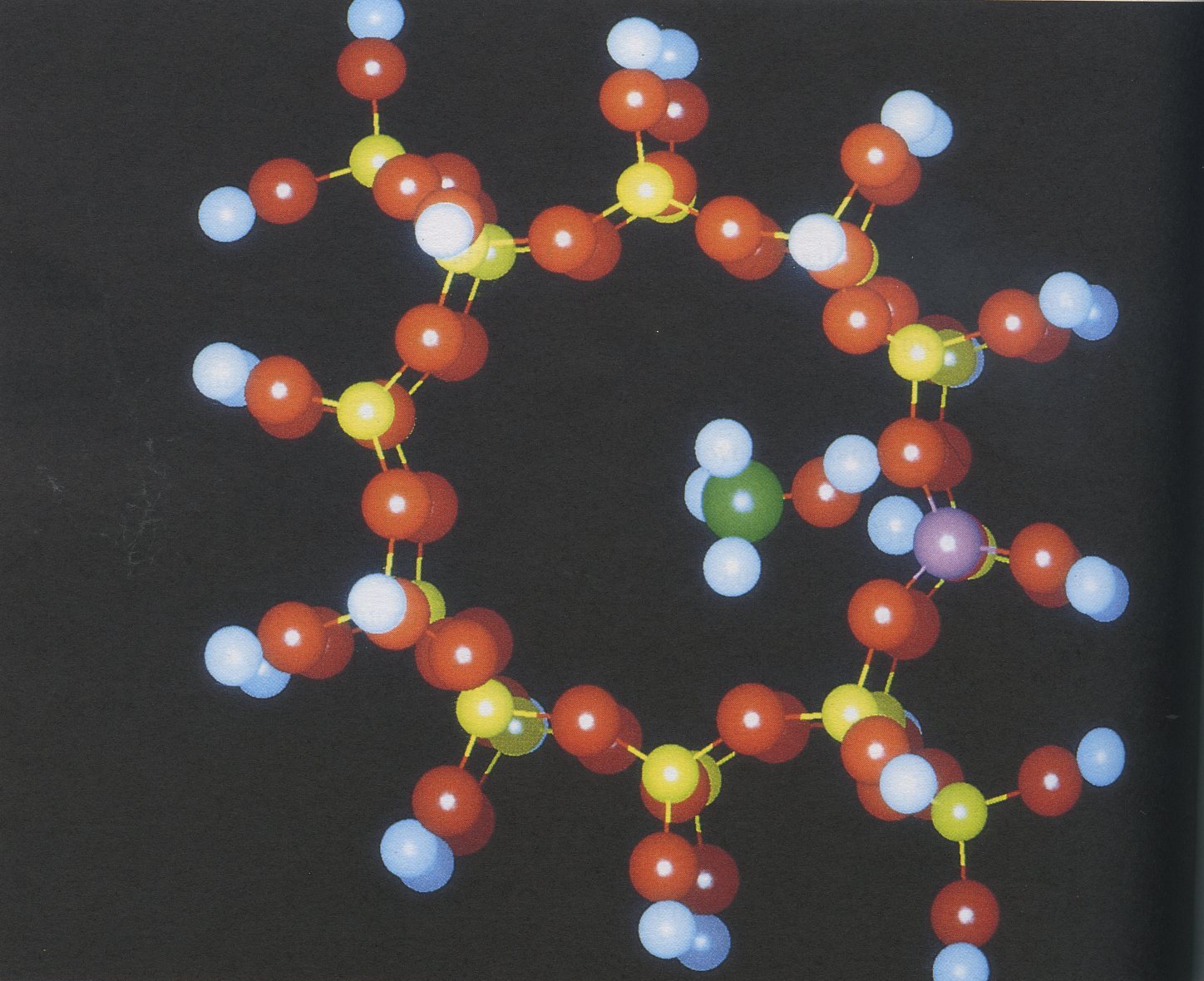
The methyl peroxy radical, CH3O2, is an important intermediate formed in the troposphere and stratosphere as part of the methane oxidation cycle 1. Recent experimental and modelling studies [2,3] have indicated that the CH3O2 radical could play an important role in the destruction of atmospheric ozone through its reaction with the ClO radical. The seven possible reaction channels for the reaction of ClO and CH3O2 are shown below.
                                         ΔHR(298)/kJmol-1    Channel
CH3O2 +  ClO → ClOO+CH3O                    -9.2                1
               OClO + CH3O                  -7.1                2
               CH2O + HCl + O2            -319                  3
               CH2OO + HOCl                118                  4
               CH3O + Cl + O2               17.6                5
               CH3Cl + O3                  -57                  6
               CH3OCl + O2                -178                  7
The only product of this reaction that has been detected experimentally is the CH2O species. The work of Simon et al. [2] has shown that this product could be produced directly through reaction channel 3 or as a secondary product of reaction channel 1. The rate constant for the reaction has been determined to be of the order of 1-4×10-12cm3molecule-1s-1 and to show a negative temperature dependence. These results indicate that the reaction may proceed via a complex reaction mechanism. In this work we report the first study of the reaction mechanism of the ClO + CH3O2 reaction using ab initio quantum mechanical techniques.
This work has been performed using the Gaussian92 [4] software package on the Cray X-MP and YMP at the Atlas Centre, Rutherford Appleton laboratory. The reaction mechanism has been studied by locating all possible stationary points on the reaction potential surface. The stationary points are then .characterized by determining the harmonic vibrational frequencies. Initially the surface was studied at .the UHF/6-31g* level. These results were then used as starting points for calculations at the MP2/6-31g* level. Table 1 gives the energies and internal coordinates of the reactants and products under consideration.
Table 1. Reactants and Products (All bond lengths in Angstrom and angles in degrees)
| UHF/6-31g* | ||||||||||
|---|---|---|---|---|---|---|---|---|---|---|
| Species | R ClO | R CH | R CO | R OO | <HCO | <H'CO | <COO | <ClOO | <OClO | E/Eh |
| CIO | 1.62 | -534.23227 | ||||||||
| CH3O2 | 1.08 | 1.42 | 1.30 | 105 | 110 | 111 | -189.20231 | |||
| ClOO | 1.70 | 1.28 | 111 | -609.00325 | ||||||
| CH2O | 1.09 | 1.18 | 122 | -113.86633 | ||||||
| CH3O | 1.08 | 1.38 | 106 | 111 | -114.42074 | |||||
| OClO | 1.46 | 116 | -608.93806 | |||||||
| MP2/6-31g* | ||||||||||
| ClO | 1.60 | -534.51887 | ||||||||
| ClOO | 1.72 | 1.28 | 113 | -609.48396 | ||||||
| CH3O2 | 1.09 | 1.45 | 1.31 | 105 | 108 | 110 | -189.66801 | |||
| CH2O | 1.10 | 1.22 | 122 | -114.19101 | ||||||
| CH3O | 1.09 | 1.38 | 106 | 111 | -114.69274 | |||||
| OClO | 1.51 | 120 | -609.47790 | |||||||
The energies of the stationary points located on the UHF/6-31g* surface are tabulated in table 2.
Table 2 UHF/6-31g* Surface.
| E/Eh | ||
|---|---|---|
| 1. | CH3O2OCl | -723.38989 |
| 2. | CH3O2ClO | -723.32932 |
| 3. | CH3O2OCl | -723.37779 |
| 4. | CH3O2OCl | -723.33539 |
| 5. | CH3O2OCl | -723.39312 |
| 6. | CH3O2OCl | -723.33943 |
Stationary points 1-4 correspond to saddle points on the reaction surface and stationary points 5 and 6 correspond to local minima. It is found that two types of transition states are formed at this level. The first results from attack at the terminal oxygen of the CH3O2 species by the oxygen atom of ClO and the second arises from attack at the same atom by the chlorine atom of ClO.
The stationary points located on the UHF surface were used as an initial guess for a study using second-order Moller-Plesset perturbation theory. The results of this work are reported in table 3.
Table MP2/6-31g* Surface.
| E/Eh | ||
|---|---|---|
| 1. | CH3O2OCl | -724.22965 |
| 2. | CH3O2ClO | -724.19402 |
| 3. | CH3O2OCl | -724.22301 |
| 5. | CH3O2OCl | -724.23294 |
| 6. | CH3O2ClO | -724.19818 |
Points 1-3 on the MP2 reaction surface were found to correspond to saddle points and the remaining points were found to be local minima on the surface. At the MP2 level no saddle point corresponding to stationary point 4 on the UHF surface could be located. The barrier heights for the stationary points located on the UHF and MP2 reaction surfaces are tabulated below in table 4.
Table 4 Barrier Heights/kJmol-1
| UHF/6-31g* | MP2/6-31g* | ||
|---|---|---|---|
| 1. | CH3O2OCl | 117 | -112 |
| 2. | CH3O2ClO | 276 | -18 |
| 3. | CH3O2OCl | 149 | -94 |
| 4. | CH3O2ClO | 260 | |
| 5. | CH3O2OCl | 108 | -120 |
| 6. | CH3O2ClO | 249 | -30 |
Table 4 shows the importance of including electron correlation in reaction mechanism studies. The barrier heights are significantly lower at the MP2 level than at the UHF level. However even at the MP2 level the computed barrier heights will still be overestimated. Improved barrier heights can be obtained by performing single point calculations, at the MP2/6-31g* optimized geometries, using higher levels of theory. However it is expected that the nature of the reaction surface will not differ dramatically from that computed at the MP2 level. At the MP2 level the large negative barrier heights indicate that the reaction probably occurs via a complex mechanism. This result is in keeping with the unusual temperature dependence exhibited by the rate constant for this reaction.
Further work is in progress to determine the reaction mechanism for the ClO + CH3O2 reaction. The work, to date, has only considered direct attack by ClO at the terminal oxygen atom of the methyl peroxy radical. Calculations will be performed to study the possibility of the formation of cyclic transition states or intermediates. Intrinsic reaction coordinates calculations are in progress to determine the relationships between the located stationary points and the reactants and products. The preliminary calculations have already shown that the reaction surface appears to have a complex structure. It can also be seen from table 4 that it is necessary to study the CH3O2 + ClO system at a high level of theory in order to obtain a reasonable description of the reaction mechanism.
1 S. W. Benson, P. S. Nangia, Acc. Chem. Res., .12, (1979), 223.
2 F. G. Simon, J.P. Burrows, W. Schneider, G. K. Moortgat, P. J. Crutzen, J. Phys. Chem., 23,, (1989); 7807.
3 P. J. Crutzen, R. Muller, Ch. Brohl, Th. Peter, Geophys. Res. Letts., 1..2, (1992), 1113.
4 Gaussian 92, Revision A, M. J. Frisch, G. W. Trucks, M. Head-Gordon, P. M. W. Gill, M. W. Wong, J.B. Foresman, B. G. Johnson, H. B. Schlegel, M. A. Robb, E. S. Reploge, R. Gumperts, J. L. Anders, K. Raghavachari, J. S. Binkley, C. Gonzalez, R. L. Martin, D. J. Fox, D. J. DeFrees, J. Baker, J. T. P. stewart, J. A. Pople, Gaussian Inc., Pittsburgh PA, 1992.
5 C. Gonzalez, H. B. Schlegel, J. Phys. Chem., 90, (1989), 2154.
Since the 1930s the first row transition metal monoxides have provided interesting challenges to commonly accepted theories of electronic structure and bonding. They exhibit wide variation in crystal structure, bonding, valence, charge and defect states, magnetism and chemical reactivity. Despite extensive experimental and theoretical study, many problems remain.
We have begun to use the CRA Y-YMP to address many of the issues central to the chemistry of such systems using ab initio Hartree-Fock calculations using extended solid-state basis sets. The choice of LCAO ab initio Hartree-Fock methodology is prompted by the fact that, despite the volume of literature on the electronic structure of the transition metal oxides based on the local density approximation, the LDA approach encounters difficulties of the sort reported by Pickett [1], whilst recent modifications such as LDA+U [2] and SIC-LSD [3] have sought to emulate some of the features of the Hartree-Fock Hamiltonian. The theoretical methodology is embodied in the periodic Hartree-Fock code CRYSTAL 92 [4,5] as implemented on the CRAY-YMP. The project involves extensive collaboration with Drs. V.R. Saunders and N .M. Harrison at Daresbury Laboratory.
We have carried out ab initio Hartree-Fock SCF calculations for VO, MnO and NiO and, as a useful reference system, CaO using extended basis sets and the UHF scheme for open shell states. In each case the atomic states in an octahedral field consist of spin-orbitals that have either zero (Ca) or full (V, Mn, Ni) occupancy so that it is sufficient to construct the appropriate Bloch function for each oxide from a single determinant of localised functions. All four oxides are found to be essentially ionic in nature with ground states that are insulating, and, in the case of VO, MnO and NiO, high-spin antiferromagnetic. The insulating nature is primarily the result of on-site inter-band Coulombic repulsion which is sufficient to open up a large band gap. Calculated lattice parameters, binding energies, bulk moduli, elastic constants and phonon frequencies for the open-shell systems compare in accuracy with those for closed-shell oxides such as Li2O, MgO and Al2O3. In the case of MnO and NiO the agreement with experiment in respect of both the energy relative to the ferromagnetic state and the structure of the magnetic cell has been most satisfactory.
Differences are found in the upper part of the valence band between VO, MnO and NiO. In VO this is predominantly V(3d) in character. In contrast, the majority weight of the upper edge of the valence bands of MnO and NiO is O(2p) rather than M(3d). This is contrary to received wisdom but is in agreement with recent density-functional calculations. It raises the important question as to the nature of the hole states in these materials, suggesting that these are likely to be predominantly of oxygen rather than metallic character. This has implications for a diverse range of properties from electronic transport to chemical reactivity, and the bonding in the higher oxides, not only of Mn and Ni, but also of Cr, Fe and Co. In the case of NiO this seems to be in accord with oxygen K-edge data for LixNi1-xO.
We are now extending these studies [6]. New projects include the electronic structure of oxides formally containing transition metals in high oxidation states (e.g., TiO2) and antiferromagnetic fluorides such as NiF2. We have also started to consider a range of problems which relate to the defect properties of the oxides are crucial to their physico-chemical behaviour.
The first of these [7] concerns the doping of NiO and MnO with formally isovalent dopants such as MgO and aims to address the effect of a non-magnetic ion of the magnetic properties and valence band structures. We are investigating the influence of substitution on the magnetic states of these oxides and structure of the 3d-bands and how these vary as a function of impurity concentration. This requires the large of large supercells such as MgNiO2, MgNi3O4, MgNi7O8 etc. and so are particularly computationally expensive. For these systems, lattice relaxation around the defect, which is often a troublesome complication, is unlikely to be significant since Mg2+ and Ni2+ have the same charge and are similar in size.
The second is a long-standing problem in solid state physics and chemistry, namely the doping of nickel oxide with lithium, for which there exists a wealth of structural, magnetic, spectroscopic and conductivity data. This study follows on- from the important results referred to earlier concerning the valence band structures of MnO and NiO. We are now examining the properties of Li-doped NiO and Li-doped MgO as a function of Li concentration. As with Mg-doped NiO, this involves the use of large unit cells. Our results for large Li concentrations (e.g., LiNiO2) show that under these circumstances the holes have oxygen character [7]. In such cases it may well be that the holes are driven to have O character by the greater coulombic stabilisation of the nearest-neighbour oxygen hole state than the more distant cation hole state. Our current studies with larger unit cells and lower Li concentrations are vital here.
The third problem concerns interfaces - (i) the surface electronic and lattice structure of NiO and (ii) MgO/NiO layered films. Unlike MgO, with which it is often compared, NiO exhibits both the {100} and {111} surfaces. The latter is intrinsically defective, while recent atomistic simulation studies [8] have suggested that the experimental morphology can be rationalised on the basis of surface non-stoichiometry involving cation vacancies and holes. It seems unlikely that such drastic alterations to the bulk lattice structure, which appear to be necessary to stabilise the {111} surface, are not accompanied by changes in the electronic structure at the surface. The studies of the electronic structures of both these low-index surfaces which are now in progress are the first time that ab initio methods have been used in such a comprehensive way to examine defective surfaces.
Goodman [9] has described the growth and characterization of an MgO film on NiO(l00). These essentially two-dimensional systems may exhibit novel catalytic behaviour. Preliminary ab initio Hartree-Fock studies of MgO layers on NiO slabs show that there is no significant flow of charge through the interface between the two oxide. The significant charge redistribution seems to be confined to simple intraatomic polarization in the oxide layers immediately adjacent to the interface.
1. W.E. Pickett, Rev. Mod. Phys., 61,433 (1989).
2. V.I. Ansimov, M.A. Korotin and E.Z. Kurmaev, J. Phys. Condensed Matter, 2, 3973 (1990).
3. A. Svane and 0. Gunnarsson, Phys. Rev. Lett., 65, 1148 (1990).
4. R. Dovesi, V.R. Saunders and C. Roetti, 'CRYSTAL 92: An ab initio HartreeFock LCAO Program for Periodic Systems', 1992.
5. C. Pisani, R. Dovesi and C. Roetti, 'Hartree-Fock ab initio Treatment of Crystalline Systems', Springer-Verlag, 1988.
6. M.D. Towler, N.L. Allan. N.M. Harrison, V.R. Saunders, W.C. Mackrodt and E. Apra, manuscript in preparation to be submitted to Phys. Rev. B.
7. M.D. Towler, N.L. Allan. N.M. Harrison, V.R. Saunders and W.C. Mackrodt, manuscript in preparation.
8. P.M. Oliver, S.C. Parker and W.C. Mackrodt, Modelling and Simulation in Materials Science and Engineering (in press).
9. M.L. Burke and D.W. Goodman, submitted to Applied Physics Letters
The forces between molecules are very important in simulations of liquids and condensed solids and in understanding processes such as solvation. Over the last decade, there have been enormous advances in our understanding of intermolecular forces, especially in molecular (as opposed to atomic) systems. However, most of these advances have dealt with pair potentials, in which only two molecules interact at any one time. This is not the situation in condensed phases, where each molecule is surrounded by several others. Under these circumstances, the pair potentials are modified by pairwise non-additive forces. If the accurate pair potentials are to be used in condensed-phase studies, we also need to understand the non-additive forces.
In the past, work on non-additive forces has concentrated on atomic systems, such as solid argon or xenon. For such systems, it is known that the most important 3-body force is the Axilrod-Teller triple-dipole term, which is the three-body analogue of the usual 1/R6 attraction between atoms at long range. However, most of the liquids and solids of real interest contain molecules rather than atoms, and very little is known about the non-additive forces between molecules.
Recent advances in molecular beams and laser spectroscopy offer a novel way of obtaining information on non-additive forces involving molecules. High-resolution spectra of Van der Waals complexes such as Ar-HF and Ar-HCl have been obtained, and have been used to obtain very precise intermolecular potentials, which include the dependence on both the intermolecular angle and the HF/HCl vibrational state. The Ar-Ar potential is also well known. Recently, the spectroscopic groups of Gutowsky (Urbana, Illinois), Saykally (Berkeley, California) and Nesbitt (Boulder, Colorado) have succeeded in measuring high-resolution microwave and infrared spectra of the trimers Ar2-HC1 and Ar2-HF. Since the pair potentials are well known, these spectra offer the possibility of testing models of the non-additive forces.
In order to make use of the new experimental data, we need to be able to calculate the energy levels of the trimers. However, the trimers are very floppy, and execute very wide-amplitude motions about their equilibrium geometries. Quantum-mechanical calculations on tetra-atomic molecules of this type are at the limits of our computational capabilities. Using the Cray X-MP and Y-MP, we have developed methods for doing such calculations, based on a large basis-set expansion in 5 degrees of freedom.
We have now begun to use the new computational methods to learn about non-additive forces. We have found that there are significant differences between the experimental spectroscopic frequencies and those predicted on the basis of pairwise additive intermolecular forces. The differences are much larger than can be explained in terms of the uncertainties in the Ar-Ar and Ar-HCl/HF pair potentials. We have found that the discrepancies cannot be explained in terms of the "traditional" types of non-additive forces such as the Axilrod-Teller interaction, even when the anisotropy of the molecules is taken into account. However, we have identified a new type of non-additive force, which does qualitatively explain the results. The new interaction arises because the electron clouds of the two argon atoms overlap and distort one another outwards, producing an "overlap quadrupole" moment. This effect was already known, but it has little effect on the interaction energy in atomic systems. However, in a molecular system, there is a substantial energy associated with the interaction between the overlap quadrupole moment and the permanent dipole moment of the HX molecule.
This general mechanism can be expected to apply in all n-body systems containing at least one molecule: the charge clouds of two of the molecules are modified when they overlap, and this changes their interaction with the remaining (polar) molecule.
We are currently working towards determining the non-additive forces in Ar2-HCl and Ar2-HF by combining the spectra of Van der Waals dimers and trimers in a large least-squares fit. The experimental groups are extending the database of measured transitions, and we are exploring the effects of different models of non-additive forces on the spectra. Once the preliminary work has been completed, the actual fitting will require very substantial computational resources.
Calculations have been performed on the rotation-vibration spectra of several small molecules including: H+ 3, H2O, H2S, H2Se and Ar - HCN. In general these calculations were used to synthesize and analyse spectra to aid laboratory, atmospheric and astrophysical observation and assignment of spectra. Traditionally the calculations have used potential energy surfaces from either ab initio electronic structure calculations or fits to a variety of experimental data. These surfaces are generally the major source of error in calculations. Recently we have developed procedures which allows us to invert experimental data to give potential energy surfaces of outstanding accuracy - approaching that of high resolution spectroscopy. This approach is computationally intensive as it involves many recalculations of the energy levels of the system. However recent algorithmic improvements in our fitting procedure which allow derivatives of the potential energy surface to be calculated directly at little extra cost, mean that highly accurate surfaces for many triatomic systems should be obtainable by this procedure. These surfaces can be used to give further spectroscopic, and other, information about the system in question.
The first surface for which high accuracy fits were obtained was H+ 3. In this case we were able to start from two available highly accurate ab initio surfaces. Fits to both H+ 3 and D+ 3 showed that the major error in the more accurate of these surfaces was due to the Born-Oppenheimer approximation which separates the (fast) motion of the electrons from the (slow) motion of the nuclei. New Born-Oppenheimer and mass dependent non-Born-Oppenheimer (adiabatic) surfaces have been constructed for these systems which represent the available data to very high accuracy. These surfaces have resulted in a number of new and re-assignments of experimental data.
Fitting is currently under way for the water molecule. In this case there is a wealth of experimental data but no current surface satisfactorily reproduces all of it. The figure depicts the wavefunction (positive amplitude in red, negative amplitude in green) of the 18th bending state of water. The plot shows the symmetric stretch ( vertically in atomic units) against the bending angle (horizontally in Radians); the cut through the wavefunction is for both OH bondlengths kept the same. White contours depict the underlying potential energy surface with the classical turning point for the state in question being given in black. It can be seen that states such as this sample large regions of the potential energy surface and thus detailed information about the surface can be obtained from their analysis.
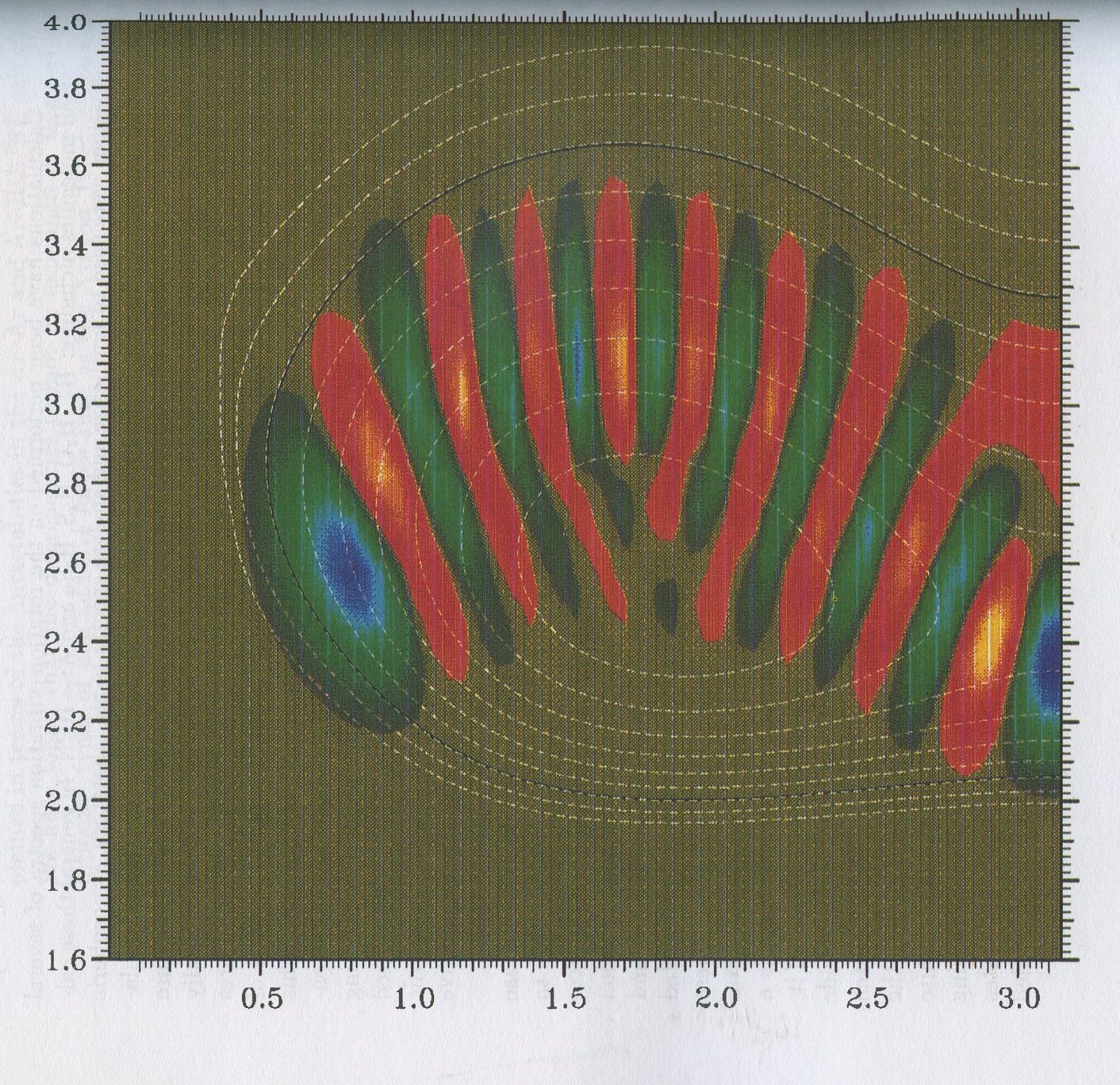
S.S. Lee, B.F. Ventrudo, D.T. Cassidy, T. Oka, S. Miller and J. Tennyson, Observation of the 3v2 → 0 overtone band of H3 +, J. Mol. Spectrosc. 145 (1991) 222
B.K. Sarpal, J. Tennyson and L.A. Morgan, Vibrationally resolved electron-HeH+ collisions using the non-adiabatic R-matrix method, J. Phys. B: At. Mol. Opt. Phys. 24 (1991) 1851
S.E. Branchett, J. Tennyson and L.A. Morgan, Differential cross sections for electronic excitation of molecular hydrogen using the R-matrix method, J. Phys. B: At. Mol. Opt. Phys. 24, (1991) 3479
B.K. Sarpal, S.E. Branchett, J. Tennyson and L.A. Morgan, Bound states using the R-matrix method: Rydberg states of HeH, J. Phys. B: At. Mol. Opt. Phys. 24, 3685 (1991) 3685
L. Kao, T. Oka, S. Miller and J. Tennyson, A table of astronomically important ro-vibrational transitions for the H3 + molecular ion, Astrophys. J. Suppl. 77 (1991) 317
J.A. Fernley, S. Miller and J. Tennyson, Band origins for water up to 22,000 cm-1 a comparison of spectroscopically determined potential energy surfaces, J. Mol. Spectrosc. 150 (1991) 597
B.K. Sarpal and J. Tennyson, Electronic transitions in the HeH molecule: a MQDT approach, J. Phys. B: At. Mol. Opt. Phys. 25, (1992) L49
K.S. Sidhu, S. Miller and J. Tennyson, Partition functions and equilibrium constants for H3 + and H2D+ Astron. Astrophys. 255 (1992) 453
J. Tennyson and B.T. Sutcliffe, Discretisation to avoid singularities in vibration-rotation Hamiltonian: a bisector embedding for AB2 triatomics, Intern. J. Quantum Chem. 42 ( 1992) 941
S.E. Branchett and J. Tennyson, Transition moments for exciation to Rydberg states of molecules using the R-matrix method: H2 with n < 5, J. Phys. B: At. Mol. Opt. Phys. 25, 2017 (1992) 2017
S. Miller, J. Tennyson and J. Fernley, Calculation of transition frequencies and line strengths of water for cool star opacities, Revista Mexicana de Astronomia y Astrofisica, 23 (1992) 63
M. Berblinger, C. Schlier, J. Tennyson and S. Miller, Accurate specific molecular state densities by phase space integration: II Comparison with quantum calculations on H3 + and HDH2 +, J. Chem. Phys. 96 (1992) 6842
B.M. Dinelli, S. Miller and J. Tennyson, Bands of H3 + up to 4v2: rovibrational transitions from first principles calculations, J. Mol. Spectrosc. 153 (1992) 718
O.L. Polyansky, S. Miller and J. Tennyson, Rotational levels of H2D+: variational calculations and assignments, J. Mol. Spectrosc. 157 (1993) 237
B.K. Sarpal, J. Tennyson and L.A. Morgan, Electron collision induced excitation and dissociation of HeH+ using the R-matrix method, in "Dissociative recombination: theory, experiments and applications", B.R. Rowe, L.B.A. Mitchell and A. Canosa (Eds.), NATO ASI series B, 165-174 (Plenum, New York, 1993).
B.K. Sarpal and J. Tennyson, Calculated vibrational excitation rates for electron -- H2 + collisions, Mon. Not. R. astr. Soc. 263 (1993) 909
J.R. Henderson, J. Tennyson and B.T. Sutcliffe, The calculation of molecular spectra using finite element methods, Phil. Mag. (in press).
L.A. Morgan and J. Tennyson, Electron impact excitation cross sections for CO, J. Phys. B: At. Mol. Opt. Phys. 26, 2429-2441.
B.M. Dinelli, S. Miller and J. Tennyson, A spectroscopically determined potential energy surface for H3 +, J. Mol. Spectrosc. (in press).
S. Miller, J. Tennyson, H.R.A. Jones and A.J. Longmore, Computation of frequencies and linestrengths for triatomic molecules of astronomical interest, in proc. 146th I.A.U. Colloquium on 'Molecular Opacities in the Stellar Enviroment', P. Thejll and U.G. Jorgenson (eds.), (Springer-Verlag, in press).
The installation of the YMP has enabled calculations to be carried out which would not have been possible using either local facilities or the XMP. The scientific areas concerned are (i) interaction of lasers with atoms, and (ii) quantum chemistry.
(i) When exposed to an intense laser field an atom may become stable against ionization. Indeed, the rate of multiphoton ionization can actually decrease with the laser intensity. This point is illustrated in Fig. 1, which is taken from the recent paper by R.M. Potvliege and P.H.G. Smith (1993, Phys. Rev. A, 48, R46) of the Physics Dept. at Durham University. The Fig. shows the lifetime of an H atom as a function of laser intensity, for two wavelengths, 620nm and 1064nm.
A comparison is made between the results of the recent calculations (solid lines) (using the YMP) and earlier, more approximate work (dashed lines). The power of the YMP was essential to this study, in which large basis sets were required to obtain accurate lifetimes at high laser intensities. It may be seen that the lifetimes are about an order of magnitude larger than had been predicted by the earlier work.
Similar studies of alkali atoms (Na and K) are currently being made and, once again, the speed and memory of the YMP are proving essential to progress in this area.
(ii) Water plays a vital role in atmospheric physics, chemistry and in biochemistry. It is also present in the interstellar medium, where it is produced in gas-phase-ion-molecule reactions or on the surfaces of interstellar grains. The theoretical study of the interactions between water molecules and other water molecules and ions requires that the electronic wavefunction of the H2O molecule should be accurately known. Recent work by Richard Wheatley (Chemistry Dept., Durham University) has been directed towards obtaining an accurate self-consistent field wavefunction by monitoring the convergence of properties, such as electric moments and polarizabilities, as the size of the basis set is increased. Very large basis sets have proved to be necessary, and the power of the YMP has been essential to the progress of these calculations.
Once an accurate SCF wavefunction has been determined, work on the properties of clusters of water molecules and ions can begin in earnest. Once again, supercomputer power will be indispensable to these studies.
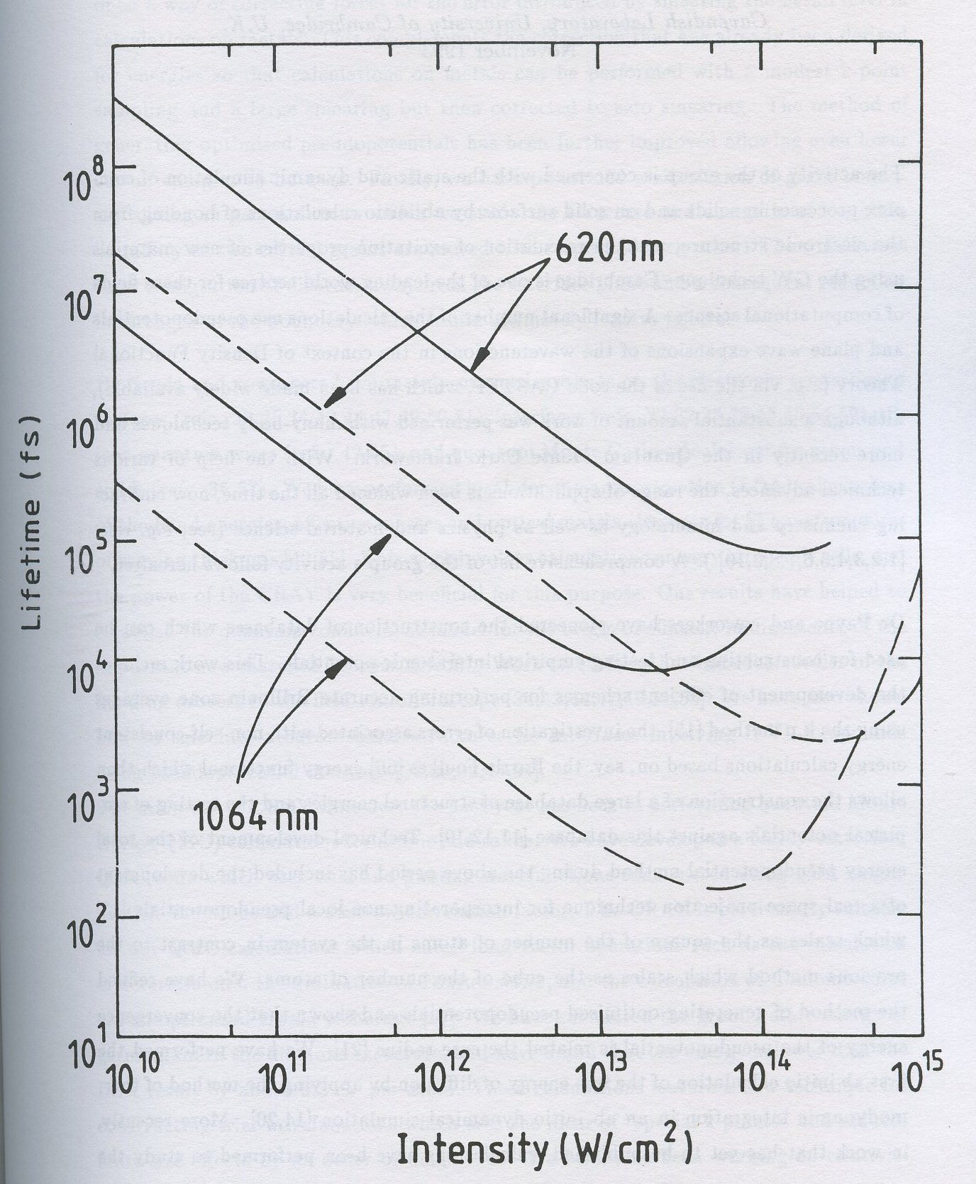
The activity of the group is concerned with the static and dynamic simulation of complex processes in solids and on solid surfaces by ab initio calculations of bonding from the electronic structure, and the calculation of excitation properties of new materials using the GW technique. Cambridge is one of the leading world centres for these fields of computational science. A significant number of the calculations use pseudopotentials and plane wave expansions of the wavefunctions in the context of Density Functional Theory (e.g. via the use of the code CASTEP, which has been made widely available), although a substantial amount of work was performed with many-body techniques and more recently in the Quantum Monte Carlo framework. With the help of various technical advances, the range of applications is been widened all the time, now embracing chemistry and mineralogy as well as physics and material science (see, e.g. refs. [1,2,3,4,5,6,7,8,9,10] ). A comprehensive list of the group's activity follows hereafter.
Dr Payne and coworkers have pioneered the construction of databases which can be used for constructing and testing empirical interatomic potentials. This work includes the development of efficient schemes for performing accurate Brillouin zone averages using the k.p method [15], the investigation of errors associated with non-self-consistent energy calculations based on, say, the Harris-Foulkes [66] energy functional which then allows the construction of a large database of structural energies and the testing of empirical potentials against this database [11,12,19]. Technical development of the total energy pseudopotential method during the above period has included the development of a real space projection technique for incorporating non-local pseudopotentials [13] which scales as the square of the number of atoms in the system in contrast to the previous method which scales as the cube of the number of atoms. We have refined the method of generating optimised pseudopotentials and shown that the convergence energy of the pseudopotential is related the core radius [21]. We have performed the first ab initio calculation of the free energy of diffusion by applying the method of thermodynamic integration in an ab initio dynamical simulation [14,20]. More recently, in work that has yet to be published, calculations have been performed to study the possibility of high temperature reconstructions on the Ge(100) surface, to calculate absolute charge densities in a range of solids and compare these to experimental results, and to calculate the polarisability of a caesium covered silicon surface. We have developed a way of correcting forces for the error introduced by smearing the Fermi level in calculations on metals. This complements the correction that has already been derived for energies so that calculations on metals can be performed with a modest k-point sampling and a large smearing but then corrected to zero smearing. The method of generating optimised pseudopotentials has been further improved allowing even lower cut-off energies to be used. Finally, we have performed a simulation of grain boundary sliding in germanium in which we study the structure and energetic of the grain boundary as two crystal grains are moved with respect to each other. The simulations show a migration of disorder away from the interface plane and a consequent reduction in strength of the boundary which would ultimately lead to failure.
Dr Needs and coworkers have mainly pursued projects on the electronic properties of surfaces (refs. 23,25,34,43,44,4 7,49,50,51), interfaces (refs. 22,32,37,38,45,46,54,59), silicon quantum wires (refs. 42,55), and quantum Monte Carlo calculations for atoms and solids (refs. 35,57). We have performed local-density approximation (LDA) calculations of the band energies, effective masses and optical matrix elements for Si quantum wires of varying thickness [42,55]. This work involves calculations on very large unit cells, and the power of the CRAY is very beneficial for this purpose. Our results have helped to establish the quantum confinement model for the origin of efficient luminescence of the important new material "porous silicon". Work on surfaces has included studies of the imaging process in the field-ion microscope [34,43,44,47,49,51,56]. We have also shown how to calculate accurate band structures for interfaces involving II-VI compounds using pseudopotential methods [22,26,32,45,54].
The main use of CRAY time over the past year has been in performing quantum Monte Carlo (QMC) calculations for atoms and solids. We have developed a highly vectorised QMC code which uses trial and guiding wavefunctions constructed using LDA single-particle functions and a Jastrow correlation factor. The CRAY is particularly suitable for our QMC calculations which entail long vector operations such as the calculation of determinants, the evaluation of Fourier series, and the calculation of Coulomb sums via an optimised Ewald technique [57]. We have calculated the ground state energy of germanium in the diamond structure, and have found that the energy is lower than the LDA result by about 0.3 eV per atom. These calculations feature a new technique for constructing trial wavefunctions which uses the ideas of "special k-points" and reduces finite-size effects by an order of magnitude. We have also been working on relativistic QMC calculations, in which we use perturbation theory to calculate relativistic corrections to the energies of atoms and solids.
The Cray supercomputers played an indispensable role in a number of projects by Dr. Godby and coworkers, in the field of computational many-body theory, allowing such quantities as the self-energy operator and dynamic screening to be calculated from first principles. In one project, various aspects of the electronic structure of the GaAs(ll0)Al semiconductor-metal interface were studied. First, attention was focused on the local quasiparticle electronic structure of the interface. The dynamic screening of the Coulomb interaction by the interface was found to give significant quantum corrections to the image-potential band-gap narrowing (38, 46]. Second, density-functional theory was used to investigate the variation of Schottky barrier height with interface structure, and the energetics of different structures. Our results have bearing on the large range of Schottky barrier heights found experimentally [59]. Another project used first-principles calculations of the self-energy of the electrons to study the dependence of the band gap of silicon on the carrier density (36].
Two projects involved the use of the Cray to study the density response of inhomogeneous systems. In one, the energies and character of low-energy charge-transfer excitations of a typical cuprate high-temperature superconductor were studied. The existence of charge-transfer excitations at the low energies that we found is an important piece of evidence in favour of their playing the central role in the mechanism for high-temperature superconductivity [63]. In the other, calculations of the inelastic X-ray scattering spectra of Be and Al were performed at different wavevectors, taking the band structure into account from first principles. Many features of the spectra, previously assigned to many-body effects, are show by this work to be artefacts of the band structure at the level of the random phase approximation [64]. Three projects were investigations of fundamental aspects of density-functional theory (DFT). In the first, Quantum Monte Carlo and non-linear optimisation techniques were used to study the exact exchange-correlation energy functional and potential for ~ model semiconducting wire, yielding information about the strengths and weaknesses of the approximations normally used [60, 62]. In the second, model calculations were used to develop a theory of the behaviour of the exact exchange-correlation potential at semiconductor interfaces (61]. In the third, the description of the metal-insulator transition in exact theory was investigated [65].
1. S Padlewski, V Heine and G D Price "Atomic order around the oxygen vacancies in sillimanite: A model for the mullite structure" Phys. Chem. Minerals 18, 373-378 (1992).
2. K.S. Chana, J.H. Samson, M.U. Luchini and V. Heine "Magnetic short range order in iron above Tc? Statistical mechanics with many-atom interactions. J Magn. Magn. Materials 104-107, 743-744 (1992).
3. K Parlinski V Heine and E K H Salje "Origin of tweed texture in the simulation of a cuprate superconductor" J. Phys. Condens. Matter sub June 1992.
4. K Parlinski, V Heine and E K H Salje "Annealing of tweed microstructure in high Tc superconductors studied by a computer simulation" sub to Acta Met. and Mater. (1992).
5. C Cheng, V Heine, R J Needs, G E Engel and I L Jones "Total Energy Calculations and related studies on SiC and ZnS polytypes" Proc. 20th International Symposium on Electronic Structure of Solids, to appear.
6. S Padlewski,V Heine and G D Price "The energetics of interaction between oxygen vacancies in sillimanite: the origin of the incommensurate structure of mullite" Phys Chem Minerals in press.
7. S Padlewski, V Heine and G D Price" A microscopic model for a very stable incommensurate modulated mineral: Mullite" sub to J. Phys. Condens. Matter Feb. 1992.
8. S.Thayaparam, M.T.Dove and V.Heine, "A Computer Simulation Study of Al/Si ordering in gehlenite and the paradox of low transition temperature" Phys. Chem. Minerals, in press
9. V.B.Deyiremenjian, V.Heine, V.Milman and M.C.Payne, "The effect of defects on the maximum tensile strength of aluminium", in press.
10. V.Heine, "Ab initio simulation of complex processes in solids" Comments Cond. Mat. Phys, submitted.
11. "Multi-atom bonding in aluminium over a wide range of coordination number" IJ Robertson, MC Payne and V Heine Europhysics Letters 15 (1991) 301.
12. "Many-atom interactions in solids" V Heine, IJ Robertson and MC Payne Phil.Trans.Roy.Soc. 334 (1991) 393.
13. "Real space implementation of non-local pseudopotentials for first principles total energy calculations" R.D. King-Smith, MC Payne and J-S. Lin Phys.Rev.B44 (1991) 13063.
14. "Ab initio static and dynamical quantum simulations: application to diffusion" V Milman, MC Payne, V Heine, RJ Needs and J-S Lin Proceedings of the APS 1991 Topical Conference on Shock Compression of Condensed Matter, Wiliamsburg, June 17-20, 1991 Eds. SC Schmidt, RD Dick, JW Forbes and DG Tasker.
15. "The k.p method in pseudopotential total energy calculations: error reduction and absolute energies" IJ Robertson and MC Payne J.Phys.Condensed Matter 3 (1991) 8841.
16. "Large scale ab initio total energy calculations on parallel computers" LJ Clarke, I Stich and MC Payne Computer Physics Communications 72 14 (1992).
17. "Ab initio total energy calculations on parallel computers: application to the Takayanagi reconstruction" MC Payne, I Stich, RD King-Smith, J-S Lin and LJ Clarke Physica Scripta T45 265 (1992).
18. "Stacking fault energies in aluminium" B. Hammer, KW Jacobsen, V Milman and MC Payne J .Phys.: Condensed Matter 4 10453 (1992).
19. "Cohesion in aluminium systems: a first principles assessment of 'glue' schemes" IJ Robertson, V Heine and MC Payne, Phys.Rev.Lett.70 1944 (1993).
20. "Free energy and entropy of diffusion by ab initio molecular dynamics: alkali ions in silicon" V Milman, MC Payne, V Heine, RJ Needs JS Lin and MH Lee, Phys.Rev.Lett.70, 2928 (1993).
21. "Optimised and transferable non-local seperable ab initio pseudotentials" J-S. Lin, A. Qteish, MC Payne and V Heine, Phys.Rev.B47, 4174 (1993).
22. Pseudopotential calculations of the valence band offsets at the ZnSe/Ge, ZnSe/GaAs and GaAs/Ge (110) interfaces: effects of the Ga and Zn 3d-electrons. A. Qteish and R.J. Needs, Phys. Rev. B 43, 4229-4235 (1991).
23. Surface stress and surface reconstruction. R.J. Needs, M.J. Godfrey and M. Mansfield, Surf. Sci. 242, 215-221 (1991).
24. The preference of silicon carbide for growth in the metastable cubic form. V. Heine, C. Cheng and R.J. Needs, J. Am. Ceram. Soc. 74, 2630-2633 (1991).
25. The surface energy and stress of Pb (111) and (110) surfaces. M. Mansfield and R.J. Needs, Phys. Rev. B 43, 8829-8833 (1991).
26. Band offset at the HgTe/CdTe (110) interface. A. Qteish and R.J. Needs, J. Phys.: Condensed Matter 3, 617-621 (1991).
27. Calculating the ground-state total energy of real systems using many-body theory. B. Farid, R.W. Godby and R.J. Needs, in Proceedings of the Workshop on Many-Body Effects in Strongly Correlated Ground States, Cambridge UK, CCP9 Newsletter, March 1991.
28. Ab initio static and dynamical simulations: application to diffusion. V. Milman, M.C. Payne, V. Heine, R.J. Needs and J.S. Lin, Proceedings of the APS 1991 Topical Conference on Shock Compression of Condensed Matter, Williamsburg VA, USA, ed. S.C. Schmidt, R.D. Dick, J.W. Forbes and D.G. Tasker, 1991.
29. Calculating optical matrix elements with non-local pseudopotentials. A.J. Read and R.J. Needs, Phys. Rev. B 44, 13071-13073 (1991).
30. A computational study into the origin of SiC polytypes. V. Heine, C. Cheng and R.J. Needs, Materials Science and Engineering B 11, 55-60 (1992).
31. Energies of atoms and solids within the local-density approximation. B. Farid and R.J. Needs, Phys. Rev. B 45, 1067-1073 (1992).
32. Improved model-solid theory calculations for valence band offsets at semiconductorsemiconductor interfaces. A. Qteish and R.J. Needs, Phys. Rev. B 45, 1317-1326 (1992).
33. Polarization, band lineups and stability of SiC polytypes. A. Qteish, V. Heine and R.J. Needs, Phys. Rev. B 45, 6534-6542 (1992).
34. Theory of the effects of image potentials on tunnelling in the field-ion microscope. S.C. Lam and R.J. Needs, Surf. Sci. 271, 376-386 (1992).
35. Green's function quantum Monte Carlo study of a jellium surface. X.-P. Li, R.J. Needs, R.M. Martin and D.M. Ceperley, Phys. Rev. B 45, 6124-6130 (1992).
36. First-principles self-energy calculations of carrier-induced band gap narrowing in silicon. A. Oschlies, R.W. Godby and R.J. Needs, Phys. Rev. B (Rapid Communications) 45, 13741-13744 (1992).
37. Electronic charge displacement around a stacking fault boundary in SiC polytypes. A. Qteish, V. Heine and R.J. Needs, Phys. Rev. B 45, 6376-6382 (1992).
38. Electronic excitation energiers in Schottky barriers. J.P.A. Charlesworth, R.W. Godby, R.J. Needs and L.J. Sham, Materials Science and Engineering B 14, 262-265 (1992).
39. The origin ofpolytypes in SiC and ZnS. V. Heine, C. Cheng, G.E. Engel and R.J. Needs, in "Wide Band-Gap Semiconductors", ed. T.D. Moustakas, J.I. Pankove and Y. Hamakawa, MRS Symposium Proceedings Vol. 242, Materials Research Society, Pittsburgh (1992).
40. Optimized norm-conserving pseudopotentials. G. Kresse, J. Hafner and R.J. Needs, J. Phys.: Condensed Matter 4, 7451-7468 (1992).
41. Structural and electronic properties of SiC polytypes. A. Qteish, V. Heine and R.J. Needs, Physica B 185, 366-378 (1993).
42. First-principles calculations of the electronic properties of silicon quantum wires. A.J. Read, R.J. Needs, K.J. Nash, L.T. Canham, P.D.J. Calcott and A. Qteish, Phys. Rev. Lett. 69, 1232-1235 (1992), Erratum, Phys. Rev. Lett. 70, 2050 (1993).
43. Calculations of ionization rate-constants in the field-ion microscope. S.C. Lam and R.J. Needs, Surf. Sci. 277, 359-369 (1992).
44. Field-ion microscope tunnelling calculations for the aluminium (111) and (110) surface, S.C. Lam and R.J. Needs, Surf. Sci. 277, 173-183 (1992).
45. Valence band offset transitivity and interface states at HgTe/CdTe, HgTe/InSb and CdTe/lnSb interfaces. A. Qteish and R.J. Needs, Phys. Rev. B 47, 3714-3717 (1993).
46. First-principles calculations of many-body band-gap narrowing at an Al/GaAs(llO) interface. J.P.A. Charlesworth, R.W. Godby and R.J. Needs, Phys. Rev. Lett. 70, 1685-1688 (1993).
47. Model-potential calculations of tunnelling rate-constants for the field-ion microscope. S.C. Lam and R.J. Needs, J. Phys.: Condensed Matter 5, 1195-1202 (1993).
48. Free energy and entropy of diffusion by Ah Initio molecular dynamics: alkali ions in silicon. V. Milman, M.C. Payne, V. Heine, R.J. Needs, J.S. Lin and M.H. Lee, Phys. Rev. Lett. 70, 2928-2931 (1993).
49. First-principles calculations of the screening of electric fields at the aluminium ( 111) and (110) surfaces. S.C. Lam and R.J. Needs, J. Phys.: Condensed Matter 5, 2101-2108 (1993).
50. Comment on "Should all surfaces be reconstructed ?" R.J. Needs, Phys. Rev. Lett. (Comments) 71, 460 (1993).
51. Imaging atoms in the field-ion microscope; tunnelling calculations using realistic potentials, S.C. Lam and R.J. Needs, accepted for publication in Phys. Rev. B.
52. First-principles calculations of the structural properties, stability and band structure of complex tetrahedral phases of germanium: ST12 and BC8. A. Mujica and R.J. Needs, accepted for publication in Phys. Rev. B.
53. Polarization, structural and electronic properties of SiC polytypes. A. Qteish, R.J. Needs and V. Heine, submitted to Computational Materials Science.
54. Ab-initio pseudopotential calculations of the valence band offset at HgTe/CdTe, HgTe/InSb and CdTe/InSb interfaces: transitivity and orientation dependence. A. Qteish and R.J. Needs, submitted to Computational Materials Science.
55. A first-principles study of the electronic properties of silicon quantum wires. R.J. Needs, A.J. Read, K.J. Nash, S. Bhattarcharjee, A. Qteish, L.T. Canham, and P.D.J. Calcott, submitted to Physica A.
56. Theory of Field Ionization. S.C. Lam and R.J. Needs, submitted to Appl. Surf. Sci.
57. An optimised Ewald method for long-ranged potentials. G. Rajagopal and R.J. Needs, submitted to J. Comput. Phys.
58. GW self-energy calculations of carrier-induced band-gap narrowing in n-type silicon. A. Oschlies, R.W. Godby and R.J. Needs, submitted to Phys. Rev. B.
59. First-principles study of the effects of interface structure on the Schottky barrier height of the Al/GaAs(ll0) interface. R.J. Needs, J.P.A. Charlesworth and R.W. Godby, submitted to Europhys. Lett.
60. "Investigating exact density-functional theory of a model semiconductor", W. Knorr and R.W. Godby, Phys. Rev. Lett. 68 639 (1992).
61. "Exchange-correlation potentials at semiconductor interfaces", R.W. Godby and L.J. Sham, to appear in Phys. Rev. B
62. "A quantum Monte Carlo study of density-functional theory for a semiconducting wire", W. Knorr and R.W. Godby, to be published.
63. "Charge-transfer excitations in cuprate superconductors", Z. Dadachanji, R.W. Godby, R.J. Needs and P.B. Littlewood, to be published.
64. "Ab-initio calculations of the dynamic response of beryllium", N.E. Maddocks, R.W. Godby and R.J .Needs, to be published.
65. "Density-functional theory of the metallisation transition of a model semiconductor", R.W. Godby and F. Gygi, to be published.
66. "Self-consistency in total energy calculations: implications for empirical and semi-empirical schemes" IJ Robertson, MC Payne, V Heine J .Phys.Condensed Matter 3 (1991) 8351.
This report is divided into two sections reflecting the different aspects of the research carried out in our group. In S1 reviews the work carried out in the last two years on molecular scattering processes while S2 focuses on atomic scattering studies over the same period.
Since the last edition of this report scientists at the Queen's University of Belfast, the University of London and the SERC Daresbury laboratory have continued to collaborate on the study of low energy electron, positron and photon collisions with molecules. The efforts in the UK are aided and abetted by international collaborations with the Harvard-Smithsonian Center for Astrophysics and the University of Minnesota in the United States, with the Institute for Physical and Chemical Science (RIKEN) in Ja pan and with the Observatoire de Paris and the University of Munster in the European Community. Members of this group perform their numerical experiments using the R-matrix approach this method being realized as a large and complex suite of computer programs. The R-matrix software has been developed from modules in the IBM Alchemy I quantum chemistry (McLean 1971) suite because the computations are closely related to the evaluation of molecular bound states. The essential feature of R-matrix theory, as depicted in figure 1, is that configuration space is divided into regions and appropriate mathematical, and therefore computational methods, are used in each region; it is the inner region which contains the molecular target and is therefore closest to a quantum chemistry problem. For technical and historical reasons, in large part associated with the evaluation of multi-centered integrals, the only targets studied so far have been diatomic molecules. As time progresses, and computers evolve, more and more complex calculations are being carried out with the software. Notwithstanding competition from the Schwinger multichannel and complex Kohn methods, developed in California, the R-matrix represents the state of the art in this field. In particular, other methods cannot compete with the R-matrix calculations for accuracy in both characterising resonance parameters and locating diffuse (Rydberg) bound states.
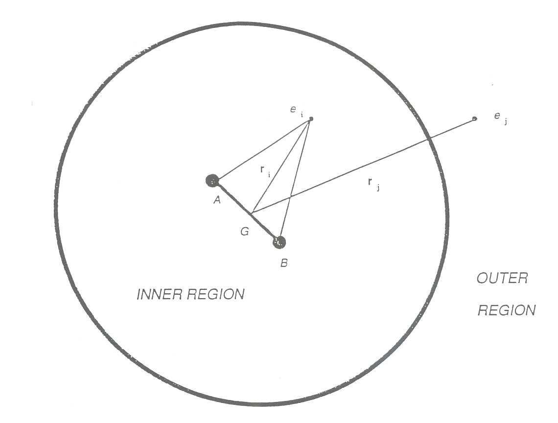
In section S1.1 the most recent applications of the program suite to diatomic targets are discussed. Specifically, it is noted that many of the computations have only been made possible by the advent of the YMP service. Section S1.2 reports on new software development for the inclusion of polyatomic targets and, finally, S1.3 considers further directions for the project. To fully appreciate the power of the R-matrix program suite and the results which it produces the reader is urged to consult the reports from the London and Daresbury groups in this volume. The strength of the combined UK effort is based upon a fruitful collaboration of the several scientists involved and exceeds, undoubtedly, the sum total of individual contributions.
The molecules O2 and N2 are of fundamental importance because they are the major components of our atmosphere. Among other applications a knowledge of data on electronic excitation by electron scattering from these targets is essential for flow field studies on high velocity projectiles re-entering the Earth's atmosphere, e.g. the Space Shuttle. Good scattering calculations are therefore essential but unfortunately represent a major challenge to computational science at this time. Fundamental to any scattering calculation is a good, but compact, representation of the molecular target states and herein lies the problem! Even the minimum acceptable representation, the Valence CI model, requires that a very large matrix be built to study the scattering. The larger memory, larger scratch disk space and faster processing power of the Y-MP/8P/128Mw service has made these computations tractable. The first ever eight state computations on these systems are now being completed and will soon be published (Gillan et al 1993, Higgins et al 1993). The data on electronic excitation of O2 has been used to compute polarization parameters for the collision of polarized electrons with the O2 molecule in its ground state; one example is shown in figure 2. Once completed data from the e-N2 work will also be used in this way.
Computing accurate cross sections for electron scattering from polar diatomic molecules continues to present theorists with a challenge. The R-matrix had already been applied to the HF and HCl targets and was recently used to carry out similar studies on e-HBr (Fandreyer et all993) This system is the first molecular target with a heavy atom to be considered by our group, the next in sequence will be e-HI. Novel software developments were required to complete the task and involved interfacing the aforementioned atomic R-matrix suite to its molecular analogues.
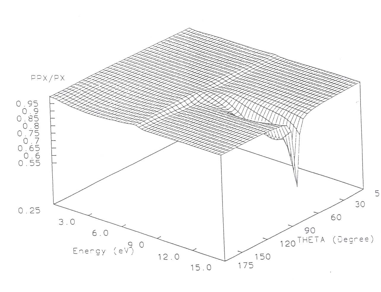
He+ 2 molecules are difficult to prepare in a laboratory and therefore it is difficult to scatter electrons from them. In this situation theory is the only tool available to the scientist who wishes to obtain data on the quasi bound states of He2 which dominate the scattering process. A lengthy series of calculations has just been completed with the R-matrix codes in which the 3Σ+ g and 3Σ+ u resonance series have been quantified and catalogued (McLaughlin et al 1991,1993). The data computed on these resonances opens the way to a host of related theoretical problems. From the results we may progress to a detailed study of Penning and associative ionization in He-He collisions, to name but one application.
Considerable effort has recently gone into extension of the algorithms and the associated codes to enable the study of electron, positron and photon scattering from polyatomic targets. It is essential to enable this facility in our codes in order to remain competitive with other research groups elsewhere in the world. When the IBM Alchemy I code was originally developed for scattering work the subroutines relating to non-linear molecules, i.e. Abelian point groups, were deleted; at the time diatomic molecules alone provided an enormous challenge. Recently the configuration generation and Hamiltonian builder subroutines, for Abelian point group molecules in Alchemy I, have been been inserted into the R-matrix codes. Since the software for integral evaluation has progressed considerably from the time that Alchemy I was written, in the Seventies, we chose not to recode it for the Cray but to use state of the art integral generator and transformation codes instead. The code MOLECULE-SWEDEN, which has been specifically optimized by its authors for the Cray architecture, was obtained, installed and the R-matrix code modified to read integrals from it. In summary the code MOLECULE-SWEDEN-ALCHEMY(R-MATRIX) was created and is now being used for molecular structure calculations. These are a necessary precursor to scattering calculations.
The final piece of software needed for scattering studies, a code which evaluates integrals between Gaussian functions and Bessel functions, is being actively developed on UNICOS. Ultimately one is required to perform millions of six dimensional integrals many of which in turn must be evaluated numerically using quadrature. Extensive studies of numerical algorithms are being carried out. An integral part of this is the use of multitasking and parallelization facilities on the machine.
The Alchemy I modules are no longer used by the computational quantum chemistry community. They are too slow for the large scale calculations which art: now commonplace in molecular structure studies. Since the R-matrix codes are being used for bigger and bigger problems we have begun to encounter the limitations of these modules more and more, this is despite some small algorithmic changes which have been introduced (Morgan and Tennyson 1993). The long term solution is to introduce the Alchemy II (McLean et al 1990) modules which are state of the art programs. With this end in sight, Queen's University have purchased a copy of the Alchemy II codes from IBM. These have been installed on the IBM 3090 at Rutherford; porting of the code to the Cray architecture is currently taking place.
When the Rutherford Cray computer was linked to the Internet and TCP/IP made available it immediately became significantly easier to access RAL when abroad. This meant that during periods spent overseas members of the group could continue to work on their usual machine obviating the need to constantly transport and install new versions of the R-matrix codes elsewhere. Additionally, however it became practical to distribute parts of calculations around the network. Partitioning of work between the newly installed Cray Y-MP/8P/128Mw-ELS at Queen's University and the Atlas Cray YMP /8P/128Mw is now commonplace.
Although the above distribution of R-matrix work was done manually it has been demonstrated by others, e.g. Alrnlof and Luthi, that automated network supercomputing can be achieved. As a result of the availability of the PVM library on the Cray Y-MP/8P/128Mw at Atlas and on the Cray YMP-ELS at Belfast (coupled with the presence of several clusters of DEC workstations on site at Queen's University) the development of parallelism in the project has been stimulated. In the near future we will develop a distributed R-matrix code and apply it to bigger systems.
With the assistance of IS and T division at Cray Research Incorporated (Minneapolis, USA) a geometry optimized structure for camphor was obtained using the UNICHEM package; this is illustrated in figure 2. Scattering of spin polarized electrons from camphor is expected to exhibit interesting effects though theorists are divided on this issue at present. Presently our group is considering the best way to tackle a calculation on this system and hope to soon report results. Hopefully we may contribute to the solution of the controversy over the magnitude of the observed effects. Clearly for a molecule of this size it will be essential to use the power of the Cray Y-MP to the full.
Almlof J and Liithi P, 1992, Chemical Physics Lett.
Gillan C J, Tennyson J and Burke P G, 1993, J. Phys B, to be submitted Higgins K B, Burke P G and Noble C J, 1993, J. Phys B, to be submitted Fandreyer R, Burke PG, Morgan LA and Gillan CJ, 1993, Proc. Roy. Soc, accepted for publication
McLaughlin B M, Gillan CJ, Burke PG and Dahler JS, 1991, Nucl. Inst. Methods, vol. B53, pp518
McLaughlin B M, Gillan CJ, Burke PG and Dahler JS, 1993, Phys Rev A, vol. 47, ppl967 McLean AD, 1971, Proc. Conf. on Potential Energy Surfaces in Chemistry edited by WA Lester Jr pub. IBM San Jose
Mc Lean A D, Yoshimine M, Lengsfield B H, Bagus P S and Liu B, 1990, Modern Techniques in Computational Chemistry, pub ESCOM-BV, ISBN 90- 72199-07-3.
Morgan LA and Tennyson J, 1993, J. Phys B, accepted for publication
UK scientists in Belfast and London, with strong support from the SERC and its supercomputing service, are prime movers in two major international projects aimed at understanding radiative and collisional processes in astrophysical plasmas: the Opacity Project, and the IRON Project.
This is an international collaboration of atomic physicists and astrophysicists. The aim was to calculate ab initio a complete set of atomic photoabsorption data required for the calculation of accurate radiative opacities for stellar envelopes.
The opacity of a plasma is a measure of the absorption of radiation by the plasma and thereby controls the transport of radiation energy. Since most of the observable universe is in the form of plasma, and moreover the production and confinement of plasma under reactor conditions is the central aim of the fusion programme, it can be seen that accurate opacity data have wide applications in different areas of physics. For example in a star. where the radiation pressure gradient balances the gravitational force in hydrostatic equilibrium, the opacity of stellar material plays a fundamental role in the structure and evolution of stars and is involved in the instabilities which lead to stellar pulsation [2,3,4]. It was here that problems first arose with the accuracy of existing opacities from Los Alamos [5], and it was clear that a reappraisal of the atomic physics and equation of state used was necessary.
By the late-nineteen-eighties a concatenation of circumstances led to the possibility of atomic physics calculations of far greater accuracy and coverage than prevously. Firstly, supercomputers had become generally available to the academic community. Secondly, atomic physicists had developed over the years powerful computational techniques for solving the collisional problem for the general atom or ion; particularly methods based on the close coupling approach such as the R-matrix method [6], which was further developed by the Opacity Project (see ADOC II [1]). And most importantly, the huge task could be shared by a number of atomic physicists worldwide who had the experience of developing and using these sophisticated software and hardware.
In stellar envelopes, typical plasma temperature, density regimes are log(K) = 6.5 to 4.5, log(g cm-3) = -1.5 to -8.5. In these conditions the isolated (unperturbed) atom approach is valid, and the dominant photoabsorption mechanisms are bound-bound and bound free transitions involving individual atoms in a complete range of excited and ionic states. Now an important feature of the R-matrix method [6] is that a single diagonalization of the Hamiltonian matrix in a local region, with suitable (bound or free wave) boundary conditions, yields the total wavefunction for any energy. The method is therefore highly efficient for sampling a large number of energies; for example when locating bound states, or when resolving the energy dependence of the photoionization process where resonances can make a significant or even dominant contribution to the absorption cross section. Both the initial (bound) and final (bound or free) states can be represented by a consistent wavefunction description, and cross sections can be calculated from any atomic or ionic ground or excited state, over any required grid of photon energies. Using these techniques, the Opacity Project was to calculate:
The atomic physics calculations were formidable; although the computer programs are now fairly automatic, handling and verifying this amount of data was a major problem. The task was finally completed in 1993 [7], and the data forms the largest, most reliable and systematic collection of atomic data ever assembled. These data are now being used to calculate multigroup and mean opacities. The expectation is that this massive infusion of high-quality atomic data into opacity calculations will lead to substantially more reliable results than are now available. The new data can also be compared with recent direct measurements of opacity using methods such as Point-Projection Spectroscopy (PPS), and with the recent calculations of the Livermore group [8], who also have used substantially improved atomic data to calculate new opacities. The entire Opacity Project data base is available in computer-readable form on computer networks, with the data server TOPBASE [9].
The Opacity Project led to many interesting atomic physics discoveries, such as the importance of 'PEC' resonances (PhotoExcitation of the atomic Core) in opacity calculations. Further developments of the atomic R-matrix method, have opened the way for a new project, concentrating on electron excitation of metal ions:
The IRON Project has the goal of computing on a large scale electron excitation cross sections and rates of astrophysical and technological importance, using the most reliable procedures currently available. Although the major effort will be for ions of the iron-group elements, other important ions will also be included. These data will complement the very extensive radiative data computed in the Opacity Project. Radiative transition probabilities not already calculated by the Opacity Project will also be provided, especially those for electric quadrupole and magnetic dipole transitions as well as for electric dipole cases in which fine structure must be taken into account.
The paucity of reliable electron excitation cross sections or rate coefficients has long hindered the quantitative analysis of astronomical spectra. Information concerning the physical state of the gas in objects for which LTE is not valid can be extracted from spectra only to the extent that collisional rates coupling the electrons to the radiating atoms and ions are known.
Because of the complexity of the Project, in particular its computational aspects, short-term and long-term goals have been identified and are being actively pursued by an international collaboration.
The first stage of the Project concerns the excitation rate coefficients for fine structure transitions in the ground configuration of astrophysically important ions in the iso-electronic sequences B, C, 0, F, Al, Si, S, and Cl. These data are essential for the interpretation of infra-red lines to be observed by the Infrared Space Observatory (ISO), as well as for coronal spectra. The calculations of fine structure and all other transitions in the ground configuration of the relevant ions are substantially completed and will be published shortly in a series of papers in A&A [10].
The second stage of the Project, which concentrates on the ions of iron, is now under way. Cross sections are now being calculated for all transitions in all ions of iron between states with principal quantum number up to at least n = 3 and when possible, to n = 4.
For some of the ions to be treated in the IRON Project, data are already available in the literature from previous close-coupling or R-matrix calculations. These data will be evaluated during the course of the Project, and if necessary recalculated with higher accuracy using the new developments of the Project, by using, for example, more accurate target wave functions, coupling to higher states, a more consistent treatment of relativistic effects, etc. A systematic approach will be used to obtain data of comparable accuracy throughout iso-electronic sequences, which has rarely been done before.
The IRON Project will use state-of-the-art theoretical and computational techniques, but will also stimulate and incorporate new theoretical developments, such as the Intermediate Energy R-Matrix (IERM) method [11], being developed in Belfast, Daresbury and Meudon. This new method allows both the valence electron and the scattering electron to be expanded in an R-matrix basis, allowing for the effects of highly lying states and ionization channels, and is the subject of current investigations.
[1] The following is a list of published papers in the Atomic Data for Opacity Calculations (ADOC) series:
ADOC I. General Description M J Seaton, J. Phys. B: At. Mol. Phys. 20 (1987) 6363-6378
ADOC II. Computational Methods K A Berrington, P G Burke, K Butler, M J Seaton, P J Storey, K T Taylor and Y Yu, J Phys. B: At. Mol. Phys. 20 (1987) 6379-6397
ADOC III. Oscillator Strengths for CII Y Yu, K T Taylor and M J Seaton, J. Phys. B: At. Mol. Phys. 20 (1987) 6399-6408
ADOC IV. Photoionization Cross Sections for CII Y Yu and M J Seaton, J. Phys. B: At. Mol. Phys. 20 (1987) 6409-6429
ADOC V. Electron Impact Broadening of Some CIII Lines M J Seaton, J. Phys. B: At. Mol. Phys. 20 (1987) 6431-6446
ADOC VI. Static Dipole Polarizabilities of the Ground States of the Helium Sequence J Thornbury and A Hibbert, J. Phys. B: At. Mol. Phys. 20 (1987) 6447-6456
ADOC VII. Energy Levels, f-Values and Photoionization Cross Sections for He-like Ions J Fernley, K T Taylor and M J Seaton, J. Phys. B: At. Mol. Phys. 20 (1987) 6457-6476
ADOC VIII. Line-Proiile Parameters for 42 Transitions in Li-like and Be-like Ions M J Seaton, J. Phys. B: At. Mol. Opt. Phys. 21 (1988) 3033
ADOC IX. The Lithium Isoelectronic Sequence G Peach, H E Saraph, and M J Seaton, J. Phys. B: At. Mol. Opt. Phys. 21 (1988) 3669
ADOC X. Oscillator Strengths and Photoionization Cross Sections for OIII D Luo, A K Pradhan, H E Saraph, P J Storey and Y Yu, J. Phys. B: At. Mol. Opt. Phys. 22 (1989) 389
ADOC XI. The Carbon Isoelectronic Sequence D Luo and A K Pradhan, J. Phys. B: At. Mol. Opt. Phys. 22 (1989) 3377
ADOC XII. Line Profile Parameters for Neutral Atoms of He, C, N and 0 M J Seaton, J. Phys. B: At. Mol. Opt. Phys. 22 (1989) 3603-3607
ADOC XIII. Line Proiiles for Transitions in Hydrogenic Ions M J Seaton, J. Phys. B: At. Mol. Opt. Phys. 23 (1990) 3255-3296
ADOC XIV. The Beryllium Sequence J A Tully, M J Seaton and KA Berrington, J. Phys. B: At. Mol. Opt. Phys. 23 (1990) 3811-3837
ADOC XV. Fe I - IV P M J Sawey and K A Berrington, J. Phys. B: At. Mol. Opt. Phys. 25 (1992) 1451-1466
[2] I Iben Jr and R S Tuggle, Astrophys. J. 197 (1975)
[3] N R Simon, Astrophys. J. (Lett) 260 (1982) 187
[4] G Bertelli, A G Bressan and C Chiosi, Astron. Astrophys. 130 (1984) 279
[5] N H Magee, A L Merts and W F Heubner, Astrophys. J. 253 (1984) 264
[6] P G Burke and K A Berrington, Atomic and molecular processes: an R-matrix approach (Institute of Physics, Bristol, England) (1993) ISBN 0-7503-0199-6.
[7] M J Seaton, Y Yu, D Mihalas and A K Pradhan, Mon. Not. R. astr. Soc. (1993) in press
[8] C A Iglesias, F J Rogers and B G Wilson, Astrophys. J. (Lett) 322 (1987) 145
[9] W Cunto and C Mendoza, Rev. Mex. Astron. Astro:fis. 23 (1992) 107
[10] D G Hummer, K A Berrington, W Eissner, A K Pradhan, H E Saraph and J A Tully, Astron. Astrophys. (1993) in press
[11] P G Burke, C J Noble and M P Scott, Proc. R. Soc. A 410 (1987) 289
Low energy electron molecule calculations have been performed for a number of diatomic targets including H+ 2 H2, HeH+, CO and N2. These calculations use R-matrix scattering codes developed by several UK institutions (London, Queen's Unversity Belfast, Daresbury) supported by Collaborative Computational Project 2. Processes studied include elastic scattering, vibrational excitation, electronic excitation and dissociate recombination (e- + HeH+ → He + H). Calculations have also been performed on bound states of the ionic systems; this method is particularly effective for studying diffuse, Rydberg states of these molecules.
Nuclear motion effects have been studied both within an approximation which separates nuclear and electronic motions, and non-adiabatic models which explicitly couples these motions. Our most advanced non-adiabatic calculations are for the dissociative recombination of HeH+. Conventional theories give effectively no cross section for this process. However we have developed a new completely non-adiabatic theory which not only gives cross sections similar in magnitude to the experiment, but also reproduces the pronounced structures observed in these experiments, see figure below.
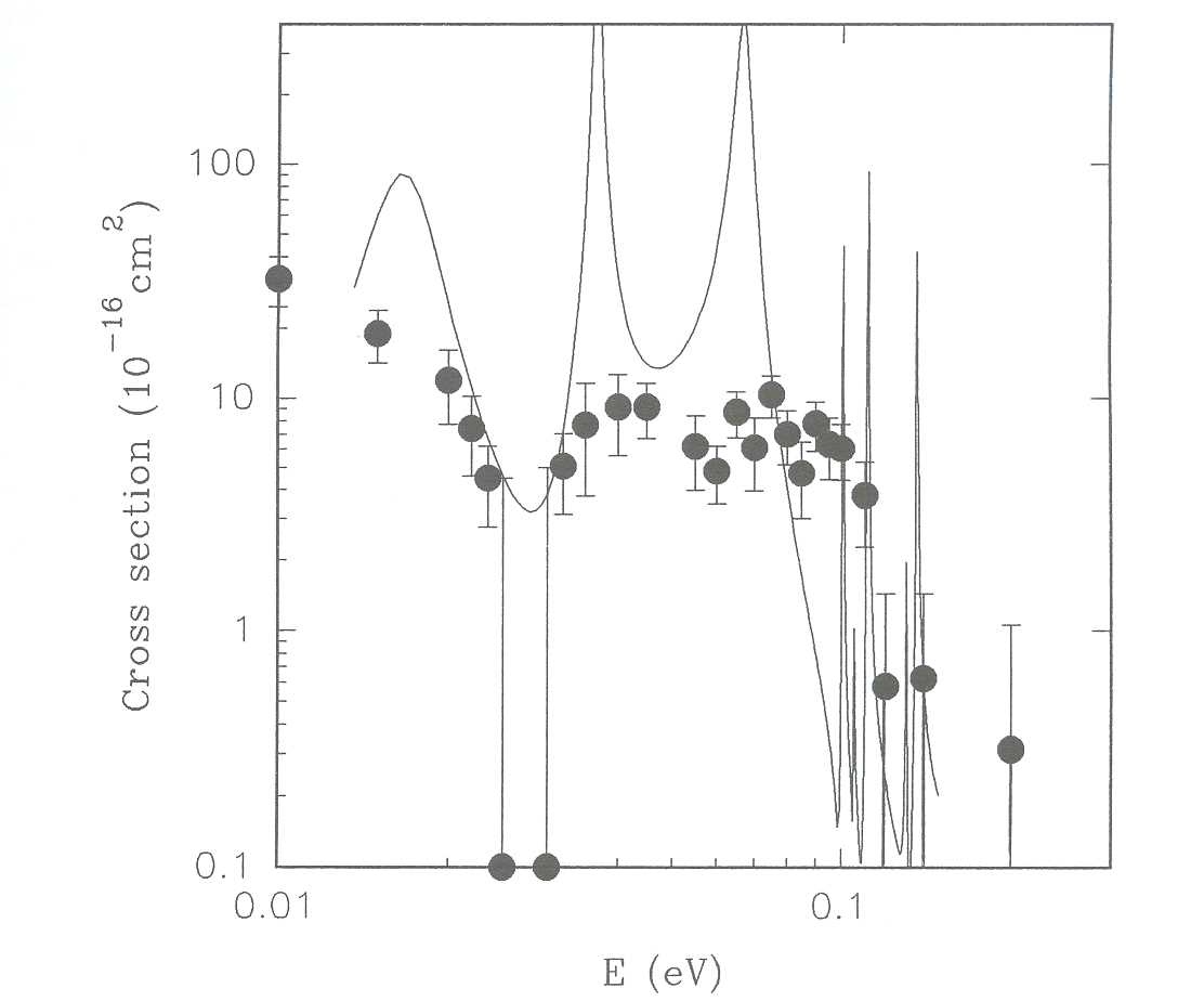
For some years now our activities have been directed towards the calculation, analysis and use of fundamental atomic data in laboratory and space astrophysics and fusion-related plasma physics and laser physics. Our work concentrates on both applied and fundamental problems concerning the accurate calculation of atomic structures and transition rates in (often highly correlated) many electron ions. We have made extensive use of three atomic structure codes: the Los Alamos suite of codes RCN/RCN2/RCG which incorporates a pseudo relativistic Hartree-Fock (HFR) model [l]; the Oxford relativistic Dirac-Feck (MCDF) structure code GRASP2 [2]; and a Multi-configuration-Hartree-Fock (MCHF) code [3]. Our work has been mainly based on use of the HFR code with the MCHF and MCDF codes often utilised to cross-check results.
Accuracy of the best ab initio atomic structure computations is limited by restrictions in the number of configuration interactions or correlation effects which can be taken into account in a computation. Many large-scale (computationally intensive) problems have been tackled which required the CRAY's processing power to deal with handling the many complex interacting configurations. We have used the HFR structure codes to gain further experience in large scale many-electron high-Z d- and f-shell shell configuration interaction (Cl) calculations [4]. Some large scale Cl studies of neutral Co, Ti and Pb structures has been undertaken in collaboration with a group in Poznan [5] as part of a program of hyperfine structure measurements and analysis. In Pb some preliminary studies of structures in the photoionization continuum have also been made [6]. Ground breaking calculations of core-excited structures in heavy atoms such as Cd in connection with (e-, 2e-) work performed in Kentucky has also been undertaken and has yielded some interesting surprises [7-8]. Some plane wave Born collision strength calculations to further this work on coherent excitation of core-excited states are also planned. Theoretical studies of E2 rates in neutral Si have been made [9], stimulated by multiphoton ionization work.
We have extended the HFR codes capabilities to handle (so far) g- and h-shell structures for up to three equivalent electrons. We also modified the code to permit computations for negative ions [10] and performed a series of feasibility tests. This development is well worth exploring further in view of the burgeoning current interest in negative ions.
We have continued to use HFR-type wavefunctions effectively in the ab initio calculation of specific mass shifts and screening effects on electron densities at the nucleus as an aid to interpreting and reconciling isotope shifts and hyperfine structures [11]. Such data are assuming increasing importance in connection wit h improvements in high resolution studies of line shapes as well as in understanding seeming anomalies in isotope abundances suggested for chemically peculiar stars.
We have continued to contribute to an extremely fruitful collaboration with heavy ion collision physicists at the GANIL facility of the University of Caen (France) in their study of photon and Auger spectra resulting from electron capture by highly charged ions. In particular C, Ar and Kr when in collision with targets such as He, H2 and Li provide a wealth of information on one-, two- and three-electron capture processes as well as new spectroscopic data for both levels and transition rates data for high n- and high l-value states of highly charged ions [12-15]. The achievement of success for such large scale studies relies very heavily on the speed and size of the CRAY.
Work towards calculating dielectronic recombination rate coefficients has continued [16,17]. This process forms the dominant recombination channel in low-density high-temperature plasmas. The study of radiative and autoionizing decay rates and of dielectronic satellite intensities for ions of astrophysical diagnostic interest continues to form a major effort. Extensive use has been made of the HFR code in the calculation of dielectronic satellite line intensities for comparison with observations of low-density, high-temperature plasmas such as occur in the solar corona and in tokamaks [18,19]. Comparison has been made in a number of studies of observed X-ray spectra from such sources, including spacecraft observations of solar flare X-ray spectra. Dielectronic satellite lines are a prominent feature of spectra below about 20 A, where a profusion occurs near the resonance lines of helium-like and hydrogen-like ions of abundant elements. The satellite intensities have a Z4 dependence, so those due to iron, calcium etc. are the most important. Their intensity ratio with the resonance line is a sensitive means of diagnosing temperature in the emitting plasma. The program DIEL within the HFR code which calculates the auto-ionization and radiative transition probabilities needed to find the intensity of an individual satellite has been used to calculate Ar XVI satellites near the He-like argon lines around 4 Angstroms which have been compared with spectra observed from the Alcator C tokamak and from solar flares. Analysis of data from a UK/US/Japan X-ray spectrometer on board the Japanese Yohkoh spacecraft will use calculations, in progress or planned, on Li-like satellites near resonance lines of helium-like S, Ca and Fe.
The interaction of high power lasers with materials usually results in the formation of a hot, dense plasma which emits radiation predominantly in the XUV and soft X-ray ranges. The Laser Plasmas group in Dublin (who in 1992 initiated the formation of an EC Network of atomic groups on the "Structure and Dynamics of Atoms and Ions") have pioneered such laser plasma studies of both emission and absorption spectra of ions of astrophysical interest. To assist analysis of these new data the codes been used in some large scale CI calculations of 2p-subshell photoabsorption spectra from ground and excited states of Mg, Al and Si ions. Work has concentrated so far on Al+ (20,21] but is being extended to include Si2+.
In addition there have been numerous (as yet) unpublished calculations made for British and Overseas Universities and Institutes and working visits have been made by co-workers from Dublin, Kansas, Kentucky, Los Alamos, Poznan and Vilnius.
1.(Univ. California Press, Berkeley,1981), (Author's description of HFR). 2 KG Dyall, IP Grant, C T Johnson, FA Parpia and E P Plummer Comput. Phys.
Commun. 58, 34 (1990); Parpia, F.A. Grant, I.P. Dyall, K.G. and Fischer, C.F. (In preparation) (Authors' description of GRASP2).
3.236 (Author's description of MCHF). J. Wiley, NY. (Author's description ofMCHF).
4. B C Fawcett and M Wilson, Computed Oscillator Strengths, Lande g-values and Lifetimes in Yb II, Atomic Data and Nuclear Data Tables 47, 241-317 (1991). RD Cowan and M Wilson,
5. J Dembczynski, E Stachowska and M Wilson Interpretation of the first spectrum of the Pb atom. 13th ICAP Munich (Aug 3-7 1992).
6. R D Cowan and M Wilson, Fano Effect in the Photoionization Cross Section of Pb. DAMOP Meeting of APS, Reno, Nevada 16-19 May 1993. Bull Amer Phys Soc 38 (3) 1150 (1993).
7. N L S Martin, D B Thompson and M Wilson, The 4d95s5p2 Autoionizing Levels of Cadmium. J Phys B: At Mol Opt Phys 24 (1991) L327-L329.
8. NL S Martin and M Wilson, The 5p6s Autoionizing Levels of Cadmium. J Phys B: At Mol Opt Phys 25 (1992) L463-L466.
9. M Wilson, Electric Quadrupole Transition Rates for Even Parity Levels of Si I, Zeit f Physik D. (1991) 21 7-10.
10. RD Cowan and M Wilson, Simple Estimates of Atomic Negative Ion Structures, Physica Scripta: 43 (1991) 244-247.
11. H-D Kronfeldt, D Ashkenasi, G Basar, L Neale and M Wilson Isotope shifts and hyperfine structures for the 5d56s7 s and 5d56s6d Configurations of Re I ( accepted for publication Oct 1992) Zeit f Physik D, Atoms, Molecules and Clusters. 25, 185-189 (1993).
12. P Boduch, M Chantepie, B C Fawcett, D Hennecart, X Husson, H Kucai, D Leder, N Stolterfoht, and M Wilson, Photon emission analysis of electron capture in 120 keV Ar8+-He or H2 collisions. Physica Scripta 45 203-211 (1992).
13. P Boduch, M Chantepie, M Druetta, B C Fawcett, D Hennecart, X Husson, H Kucal, D Leder, N Stolterfoht and M Wilson. Spectroscopic Analysis of Visible and near UV Light emitted in 120 keV l{r8+ - He and Kr8+ - H2 collisions. Physica Scripta 46 337-342 (1992).
14. P Boduch, M Chantepie, D Hennecart, X Husson, E Jacquet, D Leder, M Druett a and M Wilson, Investigation of single and double electron capture in Ar 7+ - He, H2 collisions. Physica Scripta 47,24-31 Jan (1993)
15. E.Jacquet, M Chantepie, P Boduch, M Druetta, D Hennecart, X Husson, D Leder, RE Olsen, J Pascale, N Stolterfoht and M Wilson, 120 keV Ar8+ - Li collisions studied by near UV and visible photon spectroscopy. Physica Scripta 47, 618-627 (1993).
16. K R Karim, C P Bhalla, M Ruesink, S Biel and M Wilson, Variation of dielectronic satellite intensity factors with n for 1sEl → 2lnl → 1snl dielectronic recombination processes in selected hydrogenlike ions. J Phys B: At Mol Opt Phys 24 (1991) L375-L380.
17. C P Bhalla, K R Karim and M Wilson, Angular Distribution and Linear Polarization of Photons in Dielectronic Recombination of Helium-like Ions, Nucl Inst Meths Phys Res.B56/57 (1991) 324-326.
18. K J H Phillips, F P Keenan, L K Harra, S M McCann, E Rachlew-Kallne, J E Rice and M Wilson. Calculated Ar XVII Line Intensities and Comparison with Spectra from the Alcator C Tokamak. Nucl lnstr Meths Phys Res B79 78-80 (1993).
19. K J H Phillips, L K Harra, F P Keenan, D Zarro and M Wilson, Helium-like Argon Line Emission in Solar Flares. Ap J (in press, accepted June 1993).
20. J T Costello, E T Kennedy, B F Sonntag and C W Clark, 3p photoabsorption of free and bound Cr,Cr+, Mn and Mn+, Phys Rev A 43, 1441-1450 (1991).
21. J T Costello, D Evans, R Hopkins, E T Kennedy, L Kiernan, M W D Mansfield, J-P Mosnier, M H Sayyad and B F Sonntag, 2p-subshell absorption spectra of Al+ in a laser produced plasma. J Phys B:At Mol Opt Phys 25, 5055 (1992).
L Neale and M Wilson. Ab Initio Structure of 3p4p in Si I IV ECAMP Conference, Riga, Latvia (6-10 April 1992) 16B 52.
E Jacquet, P Boduch, M Chantepie, D Hennecart, X Husson, D Leder, N Stolterfoht, M Druetta, and M Wilson. Photon Emission Analysis of 120 ke V Ar8+ - Li Collisions. IV ECAMP Conference, Riga, Latvia (6-10 April 1992) 16B 120.
P Boduch, M Chantepie, F Fremont, D Hennecart, X Husson, E Jacquet, D Leder, N Stolterfoht, M Druetta, and M Wilson. Photon Emission Analysis of 15 q-ke V Cq+ - Li Collisions. IV ECAMP Conference, Riga, Latvia (6-10 April 1992). 16B 121.
N L S Martin and M Wilson. The Effect of 5p6s on the Cd β Parameter. 23rd DAMOP meeting of APS, Chicago (20-22 May 1992) Bull Amer Phys Soc 37 (3) 1076 (1992).
D B Thompson, N LS Martin and M Wilson. Autoionizing Branching Ratios of Cd 4d95s5p2. 23rd DAMOP meeting of APS, Chicago (20-22 May 1992) Bull Amer Phys Soc 37 (3) 1135 (1992).
M Wilson. Theoretical Aspects of Recombination. NATO Advanced Research Workshop on Recombination of Atomic Ions, Newcastle Co Down, (Oct 1991) Eds: W G Graham, W Frisch, Y Hahn and J A Tanis, Plenum Press NY Sept 1992 ppl07-114. ISBN O 306 44243 4.
J Dembczynski, E Stachowska and M Wilson Interpretation of the first spectrum of the Pb atom. 13th International Conference on Atomic Physics, Munich Aug 3- 7 1992
E Jacquet, P Boduch, M Chantepie, D Hennecart, X Husson, D Leder, N Stolterfoht, M Druetta, and M Wilson. 120 keV Kr8+ - Li collisions studied by near UV and visible photon spectroscopy. 4th International Colloquium on Atomic Spectra and Oscillator Strengths for Astrophysical and Laboratory Plasmas. Sept 14-17 1992 Gaithersburg, Md. NIST Special Publication 850 Eds: J Sugar and D Leckrone, 136-138 April 1993.
F Fremont, E Jacquet, P Boduch, M Chantepie, G Cremer, D Hennecart, S Hicham, X Husson, D Leder, N Stolterfoht and M Wilson. Photon and Auger Spectroscopy of Single and Double Electron Capture following 90-keV C6+ - Li Collisions. 4th International Colloquium on Atomic Spectra and Oscillator Strengths for Astrophysical and Laboratory Plasmas. Sept 14-17 1992 Gaithersburg, Md. NIST Special Publication 850 Eds: J Sugar and D Leckrone, 139-141 April 1993.
K J H Phillips, F P Keenan, L K Harra, S M McCann, E RachlewKallne, J E Rice and M Wilson. Calculated Ar XVII Line Intensities and Comparison with Spectra from the Alcator C Tokamak. 4th International Colloquium on Atomic Spectra and Oscillator Strengths for Astrophysical and Laboratory Plasmas. Sept 14-17 1992 Gaithersburg, Md. NIST Special Publication 850 Eds: J Sugar and D Leckrone, 68- 70 April 1993.
E Jacquet, P Boduch, M Chantepie, D Hennecart, X Husson, D Leder, N Stolterfoht, M Druetta, and M Wilson. 120 keV Kr8+ - Li collisions studied by near UV and visible photon spectroscopy. Vlth International Conference on the Physics of Highly-Charged Ions, Kansas USA, Sept 28-Oct 2 (1992). AIP Confer Proc 274. Eds: P Richard et al. 163-166 (1993).
F Fremont, E Jacquet, P Boduch, M Chantepie, G Cremer, D Hennecart, S Hicham, X Husson, D Leder, N Stolterfoht and M Wilson. Photon and Auger Spectroscopy of Single and Double Electron Capture following 90-keV C6+ - Li Collisions. VIth International Conference on the Physics of Highly-Charged Ions, Kansas USA, Sept 28-Oct 2 (1992). AIP Confer Proc 274. Eds: P Richard et al. 167-170 (1993).
K J H Phillips, F P Keenan, L K Harra, S M McCann, E Rachlew- Kallne, J E Rice and M Wilson. Calculated Ar XVII Line Intensities and Comparison with Spectra from the Alcator C Tokamak. VIth International Conference on the Physics of Highly-Charged Ions, Kansas USA, Sept 28-Oct 2 (1992). AIP Confer Proc 274. Eds: P Richard et al. 441-443 (1993).
C P Bhalla, K R Karim and M Wilson. Fluorescence Yields for Hypersatellite Lines for Variously Ionized Argon. 12th lnt Conf on Appl Acee! in Res and Ind, Denton TX Nov 2-5 1992 Abstracts Eds J L Duggan and I L Morgan p38 PA35.
E Jacquet, P Boduch, M Chantepie, M Druetta, D Hennecart, X Husson, D Lecler and M Wilson Spectrocopie photonique clans le domaine 2000-6000A de la reaction Ar7+ - Li at 105 keV. Collogue du GdR 783 du CNRS Paris Jan 1993.
C P Bhalla, K R Karim and M Wilson, Fluorescence Yields for Hypersatellite Lines for Variously Ionized Silicon. DAMOP Meeting of APS, Reno, Nevada 16-19 May 1993. Bull Amer Phys Soc 38 (3) 1102 (1993).
RD Cowan and M Wilson, Fano Effect in the Photoionization Cross Section of Pb. DAMOP Meeting of APS, Reno, Nevada 16-19 May 1993. Bull Amer Phys Soc 38 (3) 1150 (1993).
L K Harra, K J H Phillips, F P Keenan and M. Wilson. Calculated He-like argon line intensities and comparison with solar flare spectra from the FCS instrument on the Solar Maximum Mission. 7th European Solar Physics meeting on "Advances in Solar Physics", Catania, Italy. (May 1993).
E Jacquet, P Boduch, M Chantepie. M Druetta, D Hennecart, X Husson, D Lecler, F Martin-Brunetiere, R E Olson, J Pascale and M Wilson. Singe electron capture following 120 keV Ne8+, Ar8+ and Kr8+ - Li collisions. 25th EGAS Caen, France 13-16 July 1993.
M Wilson, C P Bhalla and L Neale, Theoretical Autoionization Widths for the 7 sng1G4 levels in Barium 25th EGAS Caen, France 13-16 July 1993.
E Jacquet, P Boduch, M Chantepie, M Druetta, D Hennecart, X Husson, D Lecler and M Wilson. Visible and Near UV Photon Spectroscopy of Charge Exchange Collisions between Ar7+ and Li at 105 keV. 25th EGAS Caen, France 13-16 July 1993.
P Boduch, M Chantepie, G Cremer, M Druetta, D Hennecart, E Jacquet, D Lecler, F Martin-Brunetiere and M Wilson. Spectroscopic analysis of photon emission in Kr VIII spectrum. 25th EGAS Caen, France 13-16 July 1993.
P Boduch, M Chantepie, G Cremer, M Druetta, D Hennecart, E Jacquet, D Leder, F Martin-Brunetiere and M Wilson. New features of single and double electron capture processes for the 90 keV O6+ - He collision system. 25th EGAS Caen, France 13-16 July 1993.
G Basar, D Ashkenasi, D Klemz, H-D Kronfeldt, L Neale and M Wilson. Isotope shift measurements in Pt I configurations. 25th EGAS Caen, France 13-16 July 1993.
E Jacquet, P Boduch, M Chantepie. M Druetta, D Hennecart, X Husson, D Leder, F Martin-Brunetiere, R E Olson, J Pascale and M Wilson. Singe electron capture following 120 keV N e8+, Ar8+ and Kr8+ - Li collisions. ICPEAC Aarhus, Denmark July 1993.
Among the heavy fermion compounds, UPt3 exhibits many interesting properties [1]. Its unconventional superconductivity coexisting with antiferromagnetic order, the unusual antiferromagnetic order with the weak ordered moment of about 0.02 μB which doesn't show up in any bulk property, the metamagnetic transition at 22T, where the moment jumps by 0.3 μB at the U site are topics of active research.
First principles band structure calculations form a useful basis to start in understanding the properties of materials. Earlier band structure studies of UPt3 done within the local density approximation confirmed the itinerant nature of the f electrons as the predicted Fermi surface treating f electrons as valence agreed with that observed in the dHvA experiments [2]. Spin polarised calculations were performed by Norman et al [3] in the antiferromagnetic phases but the total energy of the magnetic states were not calculated. Sticht and Kubler [4] have calculated the magnetic moment and the heat of formation of UPt3 in the non-magnetic, the F and AF phases; their calculations however are not fully relativistic and spin-orbit coupling is included only in the end.
Here we report extensive band structure calculations performed on UPt3 to investigate its magnetic properties. We performed fully relativistic self-consistent electronic structure calculations of UPt3 in ( a) the observed antiferromagnetic (AF) at H = 0, (b) ferromagnetic (F) and ( c) non-magnetic phases at H =0 and at several values of the magnetic fields and obtained the following properties.
In the antiferromagnetic state at Q→ = (0.5,0,0), with moments lying in the basal plane, the unit cell doubles up. Consequently, the computations in this orthorhombic structure are extremely time consuming. With 90 k points in the irreducible wedge (IRW) of the Brillouin zone and the Hamiltonian size of 512 × 512 and two panels, the calculations required nearly 4 hours of Cray-YMP8 processor per iteration.
At H = 0, we find stable non-magnetic, ferromagnetic, as well as antiferromagnetic solutions. For comparison, all calculations were carried out in the same orthorhombic unit cell. We took particular care to obtain well converged total energies (which takes about 30 iterations in the AF case) and we also made sure the k integrations in all cases were done over the same IRW with the same number of k-points. All these solutions lie extremely close in energy within 1 mRyd/ cell of each other and moreover the non-magnetic solution has got the lowest energy. Neither the F nor AF solution is the ground state. This is unique in our experience: in all other cases if a polarised state is stable it is also the ground state.
For all further calculations in the NM and the F phases we use the smaller hep unit cell, computationally less demanding than those calculations in the orthorhombic unit cell. At H = 0, we again find that the NM solution is the ground state which confirms our earlier results in the orthorhombic structure.
In the F phase, calculations were done for different orientations of the magnetic field, along the [1120], [1010] axes in the basal plane and along [0001] direction and the ground state energies and the magnetic moments were determined.
We find the solution with the spin moment along 'a' axis is more stable than the solution with the spin moment lying along the 'c' axis by an energy difference of 0.36 mRyd. Studying this magnetic anisotropy further we also find that the in-plane anisotropy is very small, namely 0.1 mRyd. Considering the magnetic moments, small changes occur to the orbital moments: 1.48 (M∥a) and 1.:34 (M∥c). The spin moments are -1.07 (M∥a) and -1.04 (M∥c).
The electronic structure and the total energy in the F and NM phases were determined in an external magnetic field. Here the magnetic field couples only to the spin of the electrons and it is straightforward to add a term -2σ.B to the one electron Hamiltonian in our band structure calculations. As a function of the magnetic field we find the changes in the electronic structure (Fermi surface) are not significant whilst significant changes occur as a function of the direction of the field [5]. The variation of the total energy as a function of the magnetic field in the NM and F phases are shown in the following figure.
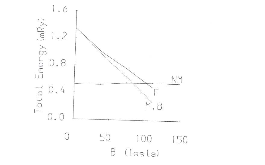
However, the important thing to note from this figure is the crossing at 102 T. Around 102 T, our calculated F solution with the moments lying along the 'a' axis crosses the non-magnetic solution and becomes the ground state. Thus a phase transition from a non-magnetic to a ferromagnetic state occurs with a jump in the net magnetic moment of about 0.4μB. Experimentally, the metamagnetic transition is obtained at 22T at which the magnetic moment jumps by 0.3μB.
The value of the critical field obtained by this method is too high. This is a consequence of the fact that the total energy calculation has overestimated the energy difference between the paramagnetic and ferromagnetic states. This is because the LDA fails to take full account of the correlations associated with the quasi-localised f electrons.
The importance of this result is that it is the first time that the metamagnetic transition in UPt3 or any other heavy fermion compound has been predicted by total energy calculation. This is a consequence of the fact that in this material the total energy calculations predict a metastable ferromagnetic phase. The calculations also predict 'a' axis to be the easy axis which is in agreement with the experiment.
Our results not only reveal the nature of the metamagnetic transition but also provide the explanation for the non-linear spin splitting of the quasi-particle bands observed by Julian et al [6].
Thus a first principles calculation carried out fully relativistically and to a high accuracy is able to explain the metamagnetic transition in a heavy fermion compound as well as to predict correctly the size of the moment in the high field state and the easy direction of the magnetisation. This is an important result because it is well known that LDA methods are successful in explaining some properties, for example Fermi surface and magnetic moments but not others, for example effective mass and photoemission line widths. This calculation shows that the extent to which the crude LDA approximation accounts for the correlations appears to be sufficient for a qualitative understanding of the rnetamagnetic transition provided the relativistic effects are treated correctly.
[l] L. Taillefer, .J. Flouquet and G.G. Lonzarich, Physica B 169 257 (1991).
[2] M.R. Norman, R.C. Albers, A.M. Boring and N.E. Christensen, Solid State Comm. 68 245 (1988).
[3] M.R. Norman, T. Oguchi and A . .J. Freeman, Phys. Rev. B 38 1119:3 (1988).
[4] J. Sticht and .J. Kubler, Sol. State Comm 54 389 (1985).
[5] M.B. Suvasini, G.Y. Guo, W.M. Ternmerman and G.A. Gehring Physica B 186-188 860 (199:3).
[6] S.R. Julian, P.A.A. Teunissen and S.A . .J. Wiegers, Phys. Rev. B 46 9821 (1992).
M.B. Suvasini, W.M. Temmerman and B.L. Gyorffy On The computational aspects of density functional theory for Superconductors Phys. Rev. B 48 (1993) 1202.
M.B. Suvasini, G.Y. Guo, W.M. Temmerman and G.A. Gehring Metamagnetic transition and electronic structure of UPt3 Physica B 186-188 (1993) 860.
M.B. Suvasini, G.Y. Guo, W.M. Temmerman and G.A. Gehring Metamagnetic transition and magnetic properties of UPt3 Submitted to Phys. Rev. Lett.
The difficulty in applying numerical techniques to quantum spin systems as opposed to classical systems is that the Hamiltonian is expressed in terms of non-commuting operators. There is consequently no simple analogue between the variables in the problem and the variables in a computer code in the same way as there might be say when solving a differential equation. This difficulty may seem at first to deny access to the plethora of useful discrete techniques that have proved so valuable for classical systems. For example Monte Carlo methods might be thought difficult to apply. How after all can the basic step of creating a new trial configuration be done with a system were the variables are operators? Fortunately this rhetorical question has now been answered by drawing on some basic results from pure mathematics which runs as follows. Suppose {Ai} are a set of bounded non-commuting operators then the following can be shown to hold
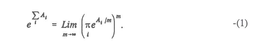
By truncating the right hand side at some large but finite value of m, which creates an error of order 1/m, the left hand side maybe approximated by a product of terms of the form eAi/m each of which can be transformed to a matrix by insertion of complete sets of states. The details of this procedure are well described in (1). Now in a classical form the right hand side of equation 1 is suitable for numerical implementation.
This procedure has been used for investigation of the thermodynamics of the spin-I chain in the presence of two-fold random anisotropy. The Hamiltonian of such a system is
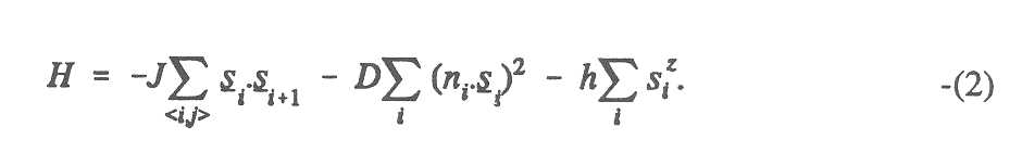
Here {Si} are spin 1 operators. {ni} are random unit vectors, D is the strength of the
anisotropy field and h is an external field. In the above J > 0 corresponds to
ferromagnetic coupling and J < 0 to antiferromagnetic coupling. Both these cases have physical interest.
For J > 0 (ferromagnetic coupling) equation 2 is a model of compounds of transition metals and rare earths.
In such substances in addition to spin-spin couplings there is at each site an easy axis of random orientation which
arises from interaction with crystal fields. This is the origin of the  in equation 2.
Using the procedure outlined above and applying the method of transfer matrices the magnetisation and susceptibility have been calculated for a range of temperatures and system sizes. The results are shown in figure 1. The significant of this plot is that there appears to be no tendency for the magnetisation to diminish as system size is increased. This indicates the irrelevance of the anisotropy. This is further indicated by a calculation of the susceptibility exponent γ which has within numerical uncertainty the value of 2. That is the same value as with D = 0. Further details can be found in [2].
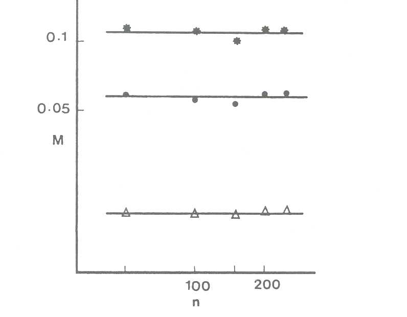
For antiferromagnetic coupling a similar approach has been adopted. Results extrapolated to zero temperature for the energy are shown in figure 2. The significance of the line with slope 2/3 is that this is the result found using first order perturbation theory and is a reflection of the singlet nature of the groundstate with D =0.
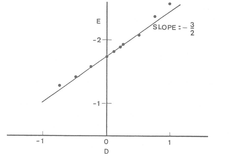
The susceptibility has also been calculated. The results are shown in figure 3. It is seen that the results for D ≠ 0 are consistent with a non-zero intercept on the T = 0 axis. This is indicative of a non-zero density of states lying above the groundstate, i.e. the Haldane gap has closed. Further particulars can be found in [3].
[1] M. Suzuki (ed). Quantum Monte Carlo Methods (Springen, Berlin) 1987.
[2] P. Reed. The Spin-1 Ferromagnetic Chain in Random Anisotropy Fields. J.Phy. A26 L807 1993.
[3] P. Reed. The Quantum Many-Body Problem in Random Fields and Anisotropies in Quantum Monte Carlo Simulations in Condensed State Physics: Lecture Notes in Physics, ed. M. Suzuki (World Scientific 1993).
The Rayleigh-Taylor (RT) instability is a widely occurring hydrodynamic phenomenon. It occurs where fluids are accelerated or sit in a gravitational field. We are studying the instability in the context of laser-produced plasmas. The Rayleigh-Taylor instability is one of the main issues determining the feasibility of Inertial Confinement Fusion (ICF). The outer surface of the ICF capsule is RT unstable as it is accelerated by the laser-generated pressure (the 'acceleration phase'). Towards the end of the implosion, the shell is decelerated (the 'deceleration phase') and is then RT unstable on the inner surface. The deceleration-phase instability can lead to loss of spherical symmetry, reduced spherical convergence and a consequent inability to reach the pr (density × radius) required for gain.
We have modelled the instability using a 3D spherical code (PLATO) which uses the symmetry of platonic solids to reduce the computational grid. A 20-sided platonic solid has 12 vertices. This symmetry is appropriate for the VULCAN laser at the Central Laser Facility if the beams are assumed to impinge on the target at the vertices of the figure. In this symmetry, the surface of a sphere can be reduced to 120 self-similar spherical triangles, thus making a large saving in the computing power needed to model an ICF implosion, although the limitations of the symmetry must be accepted. The first version of PLATO did not include diffusive transport, but it was sufficient for the modelling of the purely hydrodynamic aspects of the RT instability in the deceleration phase (Town & Bell, 1991; Town et al, 1993). Apart from similar work by Sakagami & Nishihara (1990), which came to misleading conclusions, we were the first to study the deceleration phase in 3D. We found that the non-linear RT growth in a spherically converging shell target is faster when calculated in 3D than in 2D. Depending on the shape of the initial perturbation, the geometry in 3D can either be that of a spike of shell material protruding into the fuel surrounded by a valley ( elongated bubble) of fuel rising into the shell, or conversely a bubble of fuel surrounded by a ridge (elongated spike) of shell material falling into the fuel. We showed that the bubble/ridge geometry exhibits faster non-linear growth than the spike/valley geometry. We also found that growth is faster for thin shells than thick shells.
The perturbation was constructed from a sum of twelve 6th order Legendre polynomials P6(cos θ) each with its pole at a different vertex on the platonic solid. P6 is the lowest order polynomial which does not add to zero when summed over the twelve poles. We have now applied the next non-zero Legendre polynomial perturbations P10(cos θ) & P12(cos θ). Linear growth for all modes was found to be consistent with analytic theory when account was taken of the finite density gradients (Mikaelian, 1989) in the code and spherical effects as analysed by Piesset (1954). These higher order modes were found to grow faster in the non-linear regime than expected by extrapolation from the l = 6 results. This was attributed to the growth of large bubbles at the expense of smaller bubbles (Henshaw, Pert & Youngs, 1987). This is not possible in the l = 6 case since all the bubbles have the same size.
We have shown that the time dependent growth of the perturbation amplitude does not fit a simple ηgt2 growth. Also, sudden increases in the rate of growth are seen which can be associated with shocks reflected from the centre of the target encountering the inner surface of the shell. Thus, the Richtmyer-Meshkov instability is seen to be important.
In recent months we have included laser energy absorption and diffusive transport in PLATO. We are now modelling complete ICF implosions in 3D. To our knowledge, we are the first to do this.
B J Jones, R P J Town & A R Bell
When a solid target is irradiated with a very short (psec) laser pulse, hydrodynamic expansion and heat front penetration has very little time to occur. Consequently, the temperature and density gradients remain very steep during the laser pulse, and non-local (mean free path comparable with scalelengths) transport effects have to be taken account of. A Fokker-Planck (FP) model is appropriate and practical, and we have further developed our earlier FP codes to model the extreme conditions in short pulse experiments. We find that the heat flow is much closer to the free-streaming limit than in long pulse experiments and that differences between FP and Spitzer temperature profiles are much larger.
Most recently, the code has been extended to model ionisation (Town & Bell, 1992) to give a more realistic simulation of experiments. Ionisation requires energy to be supplied to the atoms, thus reducing the temperature of the target and reducing the penetration of the heat front into the target. The degree of ionisation also affects the electron collision time. It is essential that this is included if the transport model is to be accurate.
We employed the NIMP (Non-LTE Ionisation Material Package) code (supplied by Dr S J Rose of RAL; Djaoui et al, 1992) to model the ionisation state. This is a stand-alone package which we used to post-process the FP code. The code takes as its inputs the nuclear charge, atomic weight and the time history of the temperature, density and radiation temperature (which was set to zero in our case). Collisional and radiative rates for excitation, de-excitation, ionisation and recombination are included in the model. We have modified NIMP so that we can switch off the effects of (a) radiative processes, (b) collisional excitation and deexcitation and (c) three body recombination. We can thus assess the importance of these effects on the ionisation state.
Ignoring radiative effects made no difference to the ionisation state. The absence of collisional excitation and de-excitation led to small differences in the ionisation state. In the cell with the lowest density the final ionisation state was approximately 20% smaller than when all the terms were considered. Further into the target the final ionisation state was reduced by approximately 10%. In contrast, when three body recombination was ignored the ionisation state showed a substantial departure from the exact solution. Our conclusion is that it seems reasonable to model atomic effects by including only the effects of collisional ionisation and three body recombination. These were included in the FP code. Since the FP code operates in velocity space we need cross-sections as a function of electron velocity, whereas the velocity-integrated rates are sufficient for a fluid code which models distributions which are assumed to be Maxwellian. Dr KL Bell of Belfast (Bell et al, 1983; Lennon et al, 1988) has given us much help on this matter. We find that the overlap of the cross section with the electron distribution function, from which the rate are calculated, shows only a small difference between the Maxwellian and non-Maxwellian distributions. This is encouraging for modelling of ionisation processes in FP codes since it means that the results are not usually strongly sensitive to the details of the electron distribution.
Bell KL, Gilbody HB, Hughes JG, Kingston AE & Smith FJ, Phys. Chem. Ref. Data 12, 891 (1983).
Djaoui A & Rose SJ, J. Phys. B: At. Mol. Opt. Phys. 25, 2745 appendix A (1992).
Henshaw MJdeC, Pert GJ & Youngs DL. Plasma Phys & Controlled Fusion, B29B, 405 (1987).
Lennon MA, Bell KL, Gilbody AE, Hughes JG, Kingston AE, Murray MJ & Smith FJ, Phys. Chem. Ref. Data 17, 1285 (1988).
Mikaelian KO. Phys. Rev. A, 40, 4801 (1989).
Plesset MS. J. Appl. Phys., 25, 96 (1954).
Sakagami H & Nishihara K. Phys Rev Lett, B65B, 432 (1990). Town RPJ, Bell AR. Physical Review Letters 67, 1863 (1991).
Town RPJ, Jones BJ, Findlay JD & Bell AR. submitted to Lasers & Particle Beams).
Town RP J, Bell AR. 'The importance of ionisation in short-pulse laser-plasma experiments'. Report of 1992 CECAM workshop on short pulse laser-plasma experiments.
One of the methods currently being investigated to attain controlled thermonuclear fusion as a viable energy source is Inertial Confinement Fusion (ICF). In order to achieve the fusion of two nuclei, they must collide with enough energy to overcome their mutual repulsion. This requires that the fuel, usually a deuterium-tritium gas, be contained at high temperatures (∼10keV) and high pressures (∼5x10¹⁶Pa), for a period of time long enough for the reactions to occur. In ICF, the fuel is kept in a small (∼2mm diameter) hollow spherical capsule which, in order to obtain the high temperatures and pressures required, this is symmetrically compressed using the ablation of the shell material due to incident laser beams. The compression of the capsule is required to be symmetric to within around 1% over the whole surface, and it has been shown that this requires at least 20 incident laser beams with smooth controllable intensity profiles. It is the attainment of this degree of uniformity of the laser beams that is the cause of many of the major problems in ICF today, and is the area that we have been investigating. We have been simulating this process using a 2-D hydrocode, POLLUX.
One of the main instability processes that the compressed capsule is susceptible to is the Rayleigh-Taylor instability. In its classical form, the Rayleigh-Taylor instability occurs when a heavy fluid is supported against gravity by a lighter fluid. In a general accelerating fluid system, if the density and acceleration gradients are parallel, then the amplitude of any perturbations in the density or velocity will grow due to this instability; in the small amplitude approximation, the growth of the perturbations will be exponential. Since the compression of the ICF fuel requires a high degree of spherical uniformity, any Rayleigh-Taylor growth of initial nonuniformities on the shell will cause a decrease in the yield, totally preventing ignition in the case where the growth of the nonuniformities is sufficient to break or buckle the shell. Obviously the reduction of nonuniformities on the shell and laser beams to an acceptable level is required.
Whilst target manufacturing capabilities have improved to such an extent that a sufficiently uniform shell can be constructed, the same cannot be said about the intensity profiles of current multi-stage laser beams. All multi-stage lasers have nonuniformities in their intensity profiles, be they temporal or spatial which come from slight imperfections in the various components of the system. These 'hot spots' can be imprinted on the target surface and thus create nonuniformities which will later grow as explained above. A number of methods of beam smoothing have been tried, such as induced spatial incoherence (ISI), smoothing by spectral dispersion (SSD) and the use of random phase plates (RPP). The problem with these methods is that they only provide a time averaged smoothing, but the major damage to the target occurs in the initial stages of the ablation phase when there is insufficient plasma to aid in the smoothing process, thus the problem of density nonuniformities on the target surface still exists.
In our simulations we have used a planar geometry, both to simplify the analysis and to reduce the amount of CPU time required to run the simulation. The experimental situation being simulated is simply a planar target illuminated by a laser incident from the right. The target is accelerated by the ablation of material due to the direct laser illumination. Both the laser and the target can have sinusoidal spatial modulations imposed upon them in a direction transverse to the direction of propagation of the laser beam.
Figure 1 shows the density contour plot 1200ps after the beginning of the laser pulse for a plastic foil. As can be seen from this figure, a density perturbation has been 'imprinted' on the foil by the modulated laser beam. As soon as the shock wave resulting from the initial illumination by the laser breaks through the rear of the foil (about 800ps after the laser pulse begins), the foil begins to accelerate and the system, which now consists of the foil and the ablated plasma, becomes Rayleigh-Taylor unstable thus allowing the imprinted density perturbations to grow, eventually causing the break up of the foil.
In order to quantitatively measure the imprint caused by the laser we plot the momentum perturbation. A comparative graph of momentum perturbation for three different conditions is shown in figure 2. Examining this, we see that the evolution of the system can be split into two phases, consisting of the periods before and after the shock breaks out. The second phase shows a dramatic rise in the momentum perturbation of the system, and indicates Rayleigh-Taylor growth which indirectly gives us a measure of the initial imprint. In all cases shown, the initial imprint can be seen to be large enough to cause the break-up of the target at a later stage. Quantitative investigations of the imprint of targets by a non-uniform laser for a variety of situations including shaped pulses, multi-mode laser modulations and ISI beams have been carried out by M.Desselberger et al.[1].
A novel method that we have proposed [2] and investigated in an attempt to solve the imprint problem is the use of a plasma buffer layer between the target and the laser. This layer utilises the thermal smoothing property of a plasma to smooth the laser beam nonuniformities. The laser energy in this case is absorbed at densities less than or equal to critical density in the plasma surrounding the target and is then transported to the surface of the target via electron thermal conduction which, as it is a diffusive process, smoothes any nonuniformities in the incident laser beam.
The experimental and computational set-up that we used to achieve this buffer layer consisted of the normal foil target with an attached low-density foam layer. This foam layer is pre-irradiated with soft X-rays to form the plasma buffer, before the main driving beam begins. A comparative density contour plot is shown in figure 3, for the same conditions as in figure 1. It is immediately apparent that the density perturbations present in the foil only case are absent when the pre-irradiated foam is present, a fact which is also obvious in the momentum perturbation calculations.
This method of smoothing the laser beam also has the added advantage that it does not reduce the hydrodynamic efficiency of the system, and thus decrease the possibility of ignition; allowing it to be a viable method for ICF.
The simulations described above have helped us to understand much more about the processes involved in the imprint of targets and the possible solutions to the problem, leaving us in a better position to investigate the acceleration of uniform targets.
[1] M.Desselberger et al. submitted to Journal of Applied Physics.
[2] O.Willi et al. submitted to Physical Review Letters.
M Desselberger and O Willi, Measurement and Analysis of Rayleigh-Taylor Instability in Targets driven by In coherent Lasers Phys. Fluids B 5 ( 1993) 896
O Willi, Uniformity in Direct Drive Laser Fusion: Can it be Achieved? presented at the Anomalous Absorption conference, Virginia June 1993
The quantum field theory of relativistic gauge fields interacting with matter has proved to be of tremendous importance. The theories of hadronic interactions (QCD) and of electro-weak interactions are of this type. To substantiate this identification of the relevant gauge field theories, it is clearly important to perform ab initio calculations of the properties of these theories. There are also very practical reasons to perform such calculations in order to explore the consequences of experimental data. This is because experimental results involve the interactions of the observed hadrons and these obscure the important underlying quark interactions. So it is necessary to be able to calculate the appropriate hadronic contributions in order to undertake a quantitative study of the underlying contributions - so pointing to any evidence for interactions beyond the standard model.
The only comprehensive method to perform such calculations in relativistic gauge field theory is the lattice approach. Here a (fictitious) space-time lattice is introduced and, using a finite space-time region with periodic boundaries, this gives a finite and well defined computational scheme. The scheme amounts to performing multi-dimensional integrals (in some 107 dimensions) and this can be achieved in a Monte Carlo simulation. Such a simulation then provides samples of the vacuum of the theory. Modern field theory regards the quantum fluctuations of the vacuum as giving the essence of the theory. So a study of a set of vacuum samples allows all other quantities to be estimated in principle. Indeed lattice gauge theory appears to be all about 'using a supercomputer to study nothing' but the quantum vacuum is far from empty!
Thus the way of operating is to generate vacuum samples (called configurations usually) and store them on tape. They can then be analysed repeatedly for different aspects. The UK lattice gauge theory groups at the Universities of Edinburgh, Liverpool, Southampton, Glasgow, Oxford and Cambridge combined forces to seek SERC support for a dedicated machine for these computations. A Meiko Computing Surface with 64 i860 processors was provided and sited at Edinburgh. This machine (named MAXWELL) has provided a sustained performance of over 1 Gflops and has been used continuously since its installation. Though fast at computation, MAXWELL has relatively slow input/output. This has made it appropriate to perform much of the analysis of the lattice configurations on other computers - such as the XMP and the YMP at RAL.
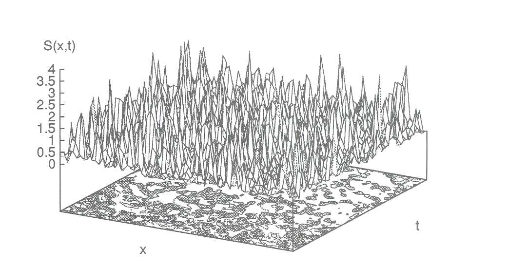
We have transferred data by posting Exabyte tapes and then copying to tape cartridges at RAL. Several projects were undertaken in this way. One of the highest profile studies was an exploration of the behaviour of the lattice method as the lattice spacing was reduced. This needed large lattices (483 × 56 was used) to retain a reasonable overall space-time size. One reason to make this study was to bridge the gap with a well-established theoretical technique which is valid at small distances: perturbation theory. Once one has been able to bridge this gap then there is no reason to take a lattice spacing any smaller. Our results show that this regime is reached. Moreover, we were able to measure the effective coupling strength of perturbation theory in terms of non-perturbative quantities such as the inter-quark potential. This effective ( or running) strength is usually quoted in terms of a dimensional scale parameter Λ. The UKQCD result is that
Λ= 256(20) MeV
in the MS bar regularisation scheme with no flavours. This is more accurate than experimental determinations, although the restriction to no flavours needs to be removed - and this is computationally a huge task for the future.
This project involved the study of the force between two quarks. Of interest to nuclear theorists is the force between two hadrons which can be explored through considering the energy of four quark systems in different geometrical arrangements. In collaboration with nuclear theorists working at Helsinki on their CRAY XMP, we have been able to measure the relatively small residual inter-hadron force in many cases of interest.
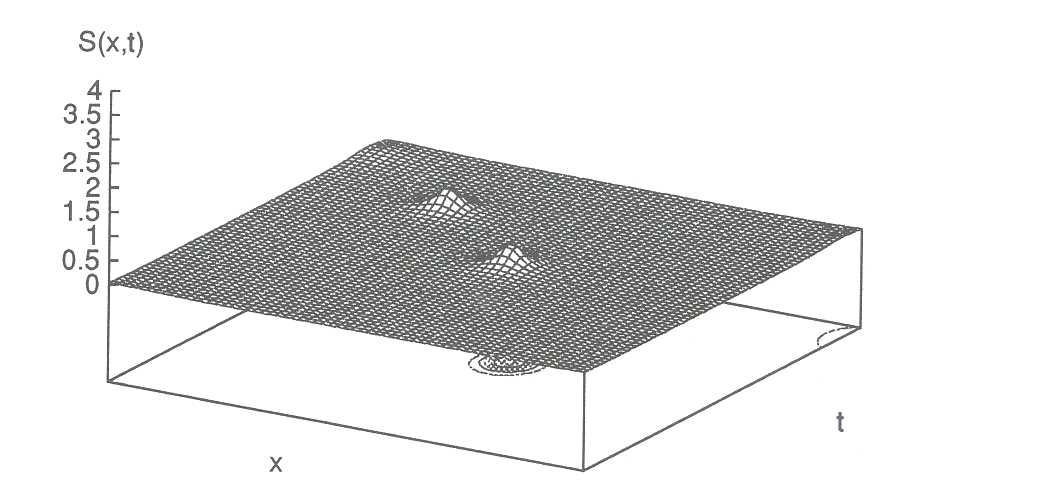
As well as QCD inspired analyses, the YMP has been used to study a simplified lattice model which mimics an interesting feature of the electro-weak theory (the standard model). This feature is that baryon number can change through special topological lattice configurations called sphalerons. Such baryon number creation or destruction processes are of utmost importance in understanding the origin of the universe. We seem to be in a universe with a net baryon number (ie not the symmetric case with as many baryons as anti-baryons) and this needs to be explained. The sphaleron configurations are extended in space and occur at the high temperatures that applied in the early universe. Their study needs non-perturbatve tools and lattice gauge theory methods have been used to explore a simplified case (in one space and one time dimension). This has enabled semi-quantitative estimates using classical techniques to be calibrated by a full ab initio lattice calculation. An extension to the full standard model is feasible but technically difficult since sphaleron contributions are expected to be very rare - a situation which is not easy to explore by stochastic simulation. Progress awaits improved algorithms for lattice study of the standard model at finite temperature.
Another study conducted at the CRAY has been to 'gauge fix' the lattice configurations. Local gauge invariance implies that the fields can be rotated in group space at each space-time point without changing any physical content. Thus it is hard to see any smooth behaviour versus space-time. The way forward is to define a smoothing criterion and to implement it iteratively. There are important theoretical reasons to study whether such 'gauge fixing' is unique and, if not, to find the properties of the multiple solutions obtained ( called Gribov copies). As well as such a study of 'gauge fixing' per se, the resulting smoothed configurations can be used to study hadronic wave functions in a very general way. This is currently in progress.
The study of topological excitations in quantum field theory has a long history. In the past, the net (integer-valued) topological charge was measured in lattice studies. It is now feasible to explore the distribution of the topological charge versus space and time. An illustration is shown of a field theory model with one space and one time dimension. The vacuum sample shows a very spiky distribution - like a bed of nails. A local smoothing enables irrelevant short-wavelength modes to be removed so exposing the underlying topological distribution. This is shown in the example where 3 instantons are present. Such studies are important because a detailed exploration of the topological density provides us with the possibility to understand the vacuum in quantum field theory - rather than just handle it as Terabyte disk files!
We present the first. set. of results for Charmonium Spectroscopy using Non-Relativistic QCD (NRQCD) on the lattice. Clear signals for the s and o hyperfine splittings have been observed as well as various orbital momentum states.
Quantum Chromodynamics (QCD) is the fundamental theory describing the interaction between quarks and gluons. A nou-perturbative solution from first. principles can be provided by lattice techniques. The application of these to bound states of heavy quarks and antiquarks, such as charrnonium states made of charm (c) quarks, offers the possibility of a stringent test. of QCD. There is a wealth of experimental data available and we are able to control statistical and systematic errors in the lattice calculation to the 10% level, a much more hopeful situation than exists for light hadron physics.
Because the internal dynamics of heavy quarkantiquark bound states is non-relativistic, we describe it with an effective theory called Nonrelativistic QCD (NRQCD). Much theoretical and numerical work has been done to develop NRQCD on the lattice [1-4]. The NRQCD Lagrangian begins with the standard terms from a non-relativistic expansion of the Dirac equation. It includes D2/2M, σ, B.2M, D, E/M2, etc. where D is a covariant derivative coupling to gluon fields. This models the important low velocity quark modes accurately. Missing high velocity quark and gluon modes appear as radiative corrections to the terms in the expansion. It turns out that the important radiative corrections are 'tadpoles', universal gluon self-interaction terms. They can be included to all orders in the coupling constant by a simple rescaling of the gluon field.
The results presented here use a Lagrangian which contains both leading and next-to-leading terms (in v2/c2) with no quark spin and leading terms with quark spin. v2/c2 is ∼ 0.3 for states. This means that splittings between different orbital states are accurate to v4/c4 i.e. 10%. Splittings between different J states at the same L, which rely on the presence of spin, are accurate to only 30%. There are other significant systematic errors present in the gluon fields from the quenched approximation. These can be estimate with a potential model and appear at the 10% level.
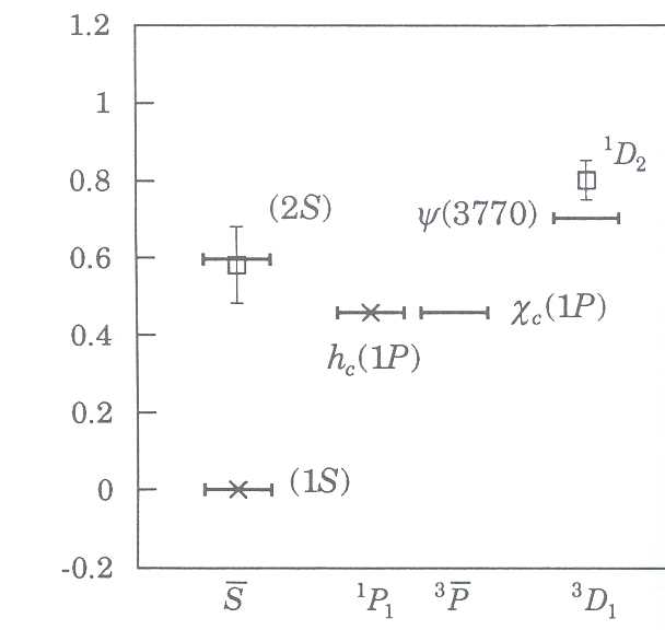
The problem must be formulated on a lattice of space-time points to solve it numerically. We discretise derivatives in the usual way and include terms in the Lagrangian to correct for discretisation errors at O(a) and O(a2) , where a is the lattice spacing. We calculate a propagator for a. heavy quark in background gluon fields generated by the UKQCD collaboration. The calculation of the propagator is an initial value problem, since heavy quarks propagate only forwards in time, and therefore relatively fast to solve.
To make a. meson we combine the heavy quark and antiquark propagators into a correlation function. Since we are working in imaginary time, the pure correlation function for a single meson decays exponentially at a rate determined by its energy (= at zero momentum, its mass). Our correlation functions reach this exponential behaviour at large times, when other excited states that they couple to have decayed away. We can then extract the mass of that meson.
All masses and splittings are in units of the lattice spacing and need to be converted to physical units (GeV). We set our result for the spin-averaged ground state P-S splitting to the experimental value to determine a. This quantity has the useful property that it is relatively insensitive to errors in fixing the quark mass. The value for a leads, via. lattice perturbation theory, to a very accurate value for the QCD coupling constant αs. The value obtained for α/MS (MZ) is 0.114 (7). The value agrees well with others extracted from comparing measured cross-sections to continuum perturbation theory.
We fix the quark mass in our Lagrangian by studying the E vs. p dispersion relation for the lightest state, called the ηc. We adjust the bare quark mass until the mass of the ηc is correct.
Figure 1 shows our results for the spin-independent splittings between different angular momentum states and radial excitations. The experimental values are indicated by horizontal bars. As described above, the 1P-1S splitting has been used to determine the scale for all the others so those states a.=re marked with a cross. A value for the mass of the excited S state, the 2S, is obtained and that agrees well with the experimental value. The mass we have calculated for a D state is for the 1D2 and it. should be rather higher than that for the experimental posited 3D1 state, the Ψ(3770).
Table 1: Results for spin dependent splittings for2S+1LJstates
| Splitting | Lattice result (MeV) | Exp (MeV) |
|---|---|---|
| 3S 1-1S0 | 96(4) | 117 |
| 3P 2-3P1 | 60(30) | 46 |
| 3P 1-3P0 | 52(9) | 95 |
Table 1 gives values for the hyperfine splittings that we calculate for 1S and 1P states, compared to their experimental values. Our results agree well within the expected 30% systematic errors.
Using Lattice NRQCD it is possible to obtain a spectrum for Charmonium in good agreement with experiment. For the bb spectrum, results are even more impressive [4]. Future calculations will reduce systematic errors further by working with unquenched gluon fields. We also plan a study of bc states as well as states combining a heavy and light quark.
This work was performed as part of the NRQCD collaboration; we thank our colleagues for many useful discussions. The calculations described here were performed on CRAY machines at the Atlas Laboratory and at the Ohio Supercomputer Centre. The configurations were generated by the UKQCD collaboration on a Meiko i860 computing surface, supported by the SERC, Meiko Limited and the University of Edinburgh. We thank the SERC for financial support for this work.
1. B.A. Thacker and G. Peter Lepage, Phys. Rev. D 43 (1991) 196.
2. C.T.H. Davies and B. A. Thacker, Nucl. Phys. 8405 (1993) 593.
3. G.P. Lepageet al, Phys. Rev. D 46 (1992) 4052.
4. NRQCD collaboration, Proceedings of LAT93 meeting, Dallas, to appear in Nucl. Phys. B (Proc. Suppl.).
This paper will describe a novel algorithm for the numerical simulation of hot collision-free plasma. The formalism is a purely general one for the solution of the collision-free Vlasov equation plus Maxwell's equations, and may be applied in principle to any space plasma simulation problem. There will be applications to laboratory plasmas, fusion plasmas and industrial plasmas where collisions may be neglected. The theoretical bases of the algorithm are strictly collision-free but collisional effects and/or velocity space diffusion may be incorporated - albeit inconveniently.
The VHS algorithm is intrinsically more efficient than PIC techniques and is a straightforward, stable and low noise algorithm. It is simpler than other Vlasov algorithms [1] and does not need to invoke artificial smoothing in velocity space. The VHS algorithm is particularly characterised by the fact that the population of simulation particles is dynamic and that the algorithm permits a flux of particles at the phase box boundary. This is particularly useful for problems such as nonlinear wave particle interactions in inhomogeneous media.
The relevant equations are Maxwell's equations and the collision-free Vlasov equation
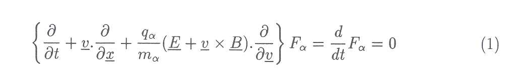
where M species α are present. Plasma charge density ρ and current density J are of course given by
Not all particle species present need be treated by VHS. Some may be described by fluid equations, or may be cold plasma/cold beams better described analytically or by PIC codes. Henceforth we shall consider only one species treated by VHS. The plasma will be described as a Vlasov or phase fluid filling a phase space of dimensionality n. Granularity of the phase fluid will be ignored. The initial distribution function F0
is required to be a regular and well behaved function of phase coordinates x, v. Discontinuities are acceptable, but delta function beams need to either be given a finite temperature or treated separately either analytically or by a PIC code.
The phase box (PSB) is constructed appropriate to the problem at hand. In general the PSB may vary with time as the simulation progresses. A phase space grid is defined, with elementary volume df = dx.dv. The grid may be inhomogeneous, non-rectilinear or indeed adaptive.
The phase space simulation box is evenly filled with simulation particles (SP's) at the start of the simulation (t = 0). At each time step each particle is pushed according to the usual equations of motion
Each particle trajectory is followed until it leaves the PSB. Trajectories are not restarted at phase space grid points as in the paper by Denavit [2]. New trajectories are continually started at the phase box boundary.
Now each SP is embedded in the phase fluid and moves with it. By Liouville's theorem each SP conserves its value of distribution function F(x, v, t). The value of F ( or δF) is thus defined on the phase trajectories of the simulation particles . During the simulation the value of F is known at a large number of points in the phase box which are the current locations of the SP's. The function of the SP's is solely to provide information. At each timestep this information is used to construct the distribution function on the fixed phase space grid and thus make estimates of the zeroth and first moments of F- which are of course plasma charge density and current density.
At each timestep we require to interpolate the values of distribution function Fl from the particles onto the fixed phase space grid, giving grid estimates Fijk ... This process of interpolation is quite different from that in PIC codes and other Vlasov codes, where charge/current or indeed distribution function are assigned or distributed to neighbouring grid points.
Once distribution function Fijk ... , is defined on the phase space grid estimates of J and ρ are readily obtained. For the 6D case
In the evaluation of the above expression it should be noted that values of Fijk ... at grid points near the boundary of the phase box will not be accurate and the moments of F are better evaluated using a smaller phase box, eliminating the boundary region.
With charge and current density defined on the spatial grid the EM fields may be pushed using standard field push techniques.
In many plasma simulation problems it might be more convenient to define the quantity δF on each phase trajectory, where

whence
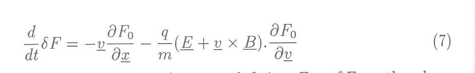
In the VHS formalism the distinction between defining F or δF on the phase trajectories is fairly trivial - hence VHS may be regarded as an algorithm that pushes δF. Note that the VHS method is not the same as a PIC code in which particles are weighted by initial distribution function. The interpolation procedure for F ensures that the available information is treated quite differently.
Clearly we need an efficient method for the interpolation of F from the particles onto the fixed phase space grid. Figure 1 shows a section of the grid of a 2D phase space simulation box. Using a derivative of the method of area weighting a suitable expression for the value of distribution function Fij at grid point ij is

where the weight factor αi for the l'th particle is given by
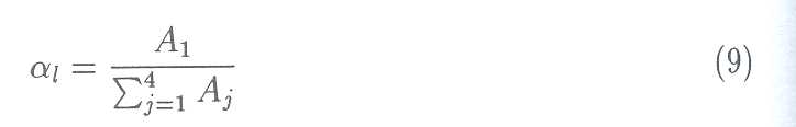
The sum is taken over all l' SP's within the 2n square area surrounding the grid point in question. The above technique will give a very low noise level in Fij and is simple and easy to encode.
A small number of grid points ij(<1 %), particularly near the phase box boundary, will not have any SP's within the surrounding 4-square area. In these cases Fij may be calculated by linear interpolation from surrounding grid points.
The expressions in equations 8 and 9 are readily generalised to the case of an n dimensional phase space. Figure 2 shows a representation of n dimensional phase space with elementary grid volume df = dx.dv.
A total of 2n hypercubes will be adjacent to grid point ij k ... If a total of l' SP's lie within this volume of phase space a suitable expression for Fijk... is given by
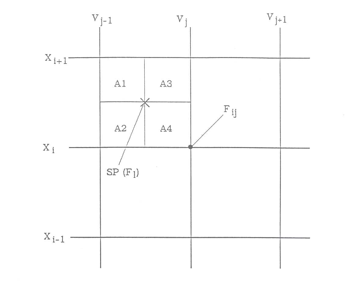
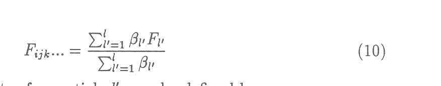
where the weighting factor for particle l' may be defined by
We first note that from Liouville's theorem the density of SP's in the phase fluid is conserved following a particle trajectory, and thus there is no tendency for SP's to bunch and leave grid point 'uncovered'. The VHS algorithm requires that 99% of all phase space grid points have at least one SP within the 2n adjacent hypercubes of volume df = dx.dv. Numerical experimentation shows that an average density ρ > ρ0 where
will give a 99.5% coverage of grid points. Note that with increasing dimensionality n, fewer SP's are needed per elementary volume df. For example for a 6D code 0.075 would suffice. To give an idea of the number of particles required by a VHS code, consider a 1 3/2D simulation with 1000 grid points in 1 spatial dimension, and 30 grid points in each of 3 velocity dimensions. The total number of SP's required would be 4.8*30*30*30*1000/16∼6M, entirely feasible with current supercomputers.
In some problems such as hot beam excitation there will be regions of phase space where F = 0. SP's need not be placed in these regions. It is only necessary to increase SP density somewhat to say 1.3 ρ0 in regions where F = 0, then al1 grid points ijk ... with no SP's in the surrounding 2n hypercubes may be regarded as having Fijk... = 0.
It must be emphasised that SP density ρ0 is a minimum value. Due to the nature of the interpolation procedure higher densities are permitted. Increased densities incur a larger computational workload but give fewer missed grid points, lower noise levels and better averaging over distribution function fine structure. This tolerance of variable density of SP's in the phase fluid makes it relatively easy to incorporate a flux of phase fluid at the phase box boundary.
A VHS code needs to control the particle population such that ρ > ρ0 everywhere, and the total population of SP's N, is within certain bounds. Figure 3 shows a representation of a 2D phase box. Over parts of the phase box boundary phase fluid will be flowing out. SP's embedded in the fluid will leave the phase box. These particles are by definition now located in an unimportant region of phase space and are providing information not required. These particles are discarded from the simulation. Conversely over parts of the phase box boundary phase fluid will be flowing in. New SP's must be inserted into this fluid. At every timestep all grid points on or near the phase box boundary are examined. New particles are inserted where there are no SP's in adjacent hypercubes. This must be done with care. The exact positions of insertion determine the resulting density in the incoming fluid.
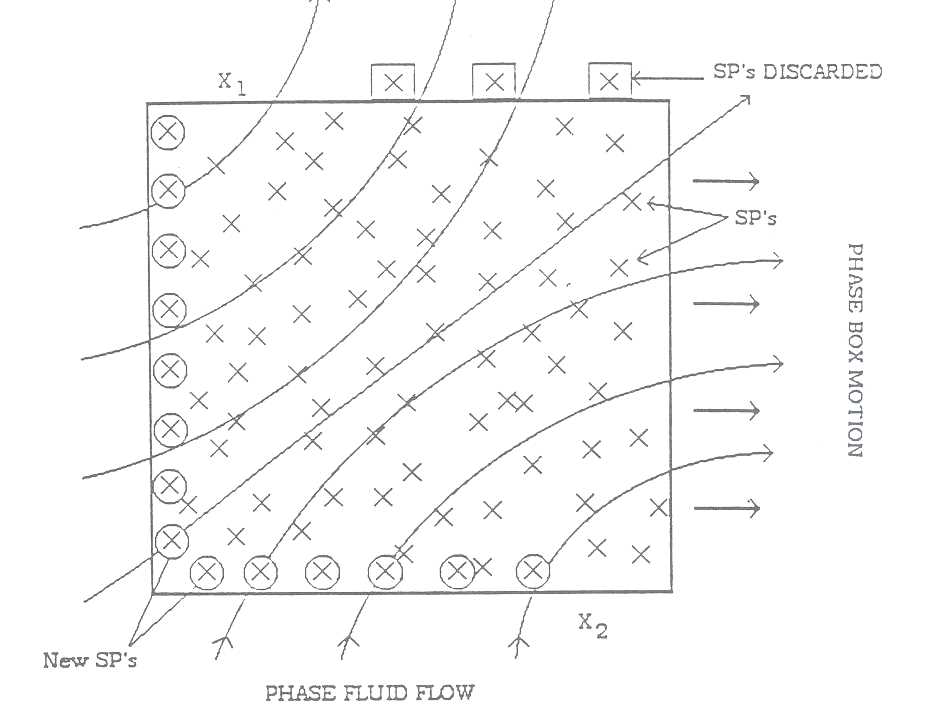
The VHS algorithm is characterised by a dynamic particle population. The total number of SP's N, will fluctuate as the simulation progresses. The algorithm is highly efficient since only particles in important regions of phase space are followed. Thus for example in wave particle interaction simulations non resonant particles will be outside the current phase box and will be discarded from the simulation. The total N, needs to be kept within reasonable bounds, say
where Nc is the number of hypercubes in the phase box. If N, falls too low inaccuracy will increase and uncovered grid points will result. The solution is to create new particles in the interior of the phase box at grid points that have 1 or O "adjacent" particles. If N, becomes too large the program will slow up and memory requirements will increase. The remedy here is to remove particles from the phase box interior where SP density is high. In the demonstrator application it was found that these measures were not necessary and that N, was adequately controlled by careful insertion of new particles at the boundary.
Where the phase space grid is inhomogeneous it will of course be necessary to create or delete particles at internal boundaries between regions of different grid density.
There will exist a wide variety of problems where the flux of phase fluid at the box boundary will be negligible and where F = 0 on the boundary. In these cases the simulation may proceed with a fixed population Nt, provided that the initial density is raised to ,..._, l.2ρ0 so that grid points with no local SP's may safely be assumed to correspond to F = 0.
At t = 0 simulation particles are given a value for distribution function of F = F0, where F0 should be self consistent with the presumed initial fields. New SP's inserted into the phase fluid need to be assigned a value for F. For insertions at the phase box boundary F = F0 is often quite sufficient. If the simulation turns out to be unduly sensitive to the choice of F for new particles, this is probably symptomatic of a phase box that is too small. In certain cases a better value for F may be available. In the VLF problem to be described a linear expression for F derived from the EM field history is used. Where a new particle is inserted into the interior of the phase box an initial value for F is readily secured by interpolating from neighbouring grid values Fijk... .
In many plasma simulations the distribution function may develop fine structure in phase space. For example this occurs with nonlinear Landau resonance when resonant particles make many oscillations within the potential trap. Usually fine structure does not have a great deal of physical significance since during the evaluation of J/ρ it will be averaged out. However fine structure can be a considerable nuisance for Vlasov codes. Other Vlasov codes such as that of Denavit [2] and Cheng and Knorr [1] need to be stabilised by filters that smooth out fine structure. The VHS method however is intrinsically stable against fine structure, since no attempt is made to evaluate derivatives of F in phase space. The VHS method does not smooth distribution function. This is considered neither desirable nor necessary.
During the 1970's and 1980's a number of papers were written reporting successful simulations using Vlasov type methods. Two methods stand out. The first is that of Cheng and Knorr [1] who numerically integrate the Maxwell/Vlasov set of equations. Particles are not used at all in this process. Because of distribution function fine structure the algorithm is complex and only stabilised by a non physical smoothing in phase space. Flux of phase fluid at the box boundary is possible but was not considered.
Denavit [2] uses particles to time advance distribution function defined on a phase space grid. Particles are started off at phase space grid points and assigned appropriate values of F. After M timesteps the values of F defined on particles are assigned to nearest grid points. This effects a reconstruction of F on the phase space grid and invokes artificial diffusion. In the limit of M = 1 reconstruction occurs at every timestep, and phase fluid flux at the phase box boundary may be accommodated but this was not considered.
A third method by Kotschenreuther [4] resembles a PIC code except that δF is pushed". Kotschenreuther noted that when δF ≪ F0 PIC codes are extremely noisy and inefficient and strongly outperformed by Vlasov codes.
It is worth summarising the advantages of the VHS method at this point. These are
The demonstrator application is a space plasma simulation in the VLF band at 3-4kHz. The code is a simulation of rising frequency emissions triggered by narrow band VLF pulses transmitted from the VLF facility at Siple, Antarctica [3]. Triggered emissions result from nonlinear electron cyclotron resonance in the equatorial region of the earth's magnetosphere at L = 4.1 The ambient hot electron distribution function is anisotropic and unstable and of a loss cone type. Cyclotron resonant energies are of order keV.
For full details of the VLF emission problem the reader is referred to Nunn [5]. Figure 4 shows the result of the simulation of the triggering of a VLF rising frequency emission by a Siple pulse. The result is presented as a frequency-time plot and bears remarkable agreement with satellite observations from space.
The computer code has been run on the Cray XMP and Cray YMP at Rutherford Laboratory. Each timestep takes about 2 seconds on the latter machine. The code uses about ½ million particles and a full simulation takes about 1 hour of Cray time. All computationally intensive parts of the code vectorise CPU, and the code has a parallelism of 512 corresponding to the ID spatial grid size. The code would run very effectively on a massively parallel machine such as the Meiko CS2.
A new algorithm has been devised for the numerical simulation of hot collision-free space plasmas. It is very efficient, low noise, stable and simple to use. Here it has been applied to the triggered VLF emission problem. It is expected that there will be many applications throughout space physics, particularly in the area of wave particle interactions.
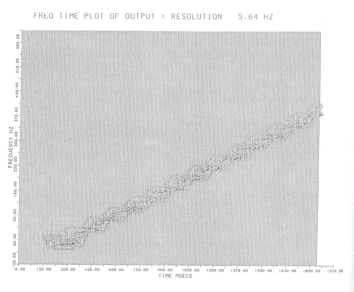
1. C. Z. Cheng and G. J. Knorr, Computational Physics, 22, 380, 1976.
2. J. Denavit, Physics of Fluids, 28 (9), 2773, 1972.
3. R. A. Helliwell and J.P. Katsufrakis, J Geophysical Research, 79, 2511, 1974.
4. M. Kotschenreuther, Physics Abstracts, 33 (9), 2107, 1988.
5. D. Nunn, Computer Physics Communications, 60, 1, 1990.
A novel technique for the numerical simulation of hot collision free plasma-- Vlasov Hybrid Simulation. J of Computational Physics vol 108 # 1 ,pp 180-196.
The problems which are confronted in astrophysics are some of the most challenging of science. Understanding the operation of astrophysical objects, such as stars and galaxies, depends on explaining physical phenomenae at energies and scale lengths which are difficult to comprehend from a merely terrestrial view point. Astronomical observations have given us a staggering range of phenomena, all of which we seek to explain, the special cases as well as the generic. The search for explanations has led to many radical ideas, and much theoretical progress has been made with appropriate simplifications. But, increasingly as observations are refined, one finds that simplified theories do not provide convincing explanations. Thus, as in other fields, astrophysicists have turned to supercomputing to advance the state of knowledge.
The usual stereotype of astrophysics is that it is a study based on remote, and rather incomplete, observations. But there is an area of astrophysics where it might truly be said we are looking in our own back yard:- space plasma physics. The Earth is immersed in plasma: The Sun produces the solar wind, a hot, fast flowing plasma which sweeps out through the solar system. The Earth is surrounded by the ionosphere, essentially a plasma of terrestrial origin. The Earth has an intrinsic magnetic field, which interacts with the magnetic field and plasma of the solar wind. All the planets have different kinds of interaction with the solar wind depending on their magnetic field. Furthermore, the solar wind undergoes its own evolution associated with changes in the source regions in the sun's corona. Interplanetary shocks can be be formed by changes in the solar wind speed, or by coronal mass ejections.
Two interesting facts make the solar wind a fascinating subject of study. Firstly, the solar wind plasma is collisionless, i.e., collisions between the constituent particles are extremely rare. Consequently, any transfer of energy and momentum, or any dissipation, has to rely on non-collisional processes which involve waves in the electric and magnetic fields. The resulting complexity makes for a number of challenging problems. Secondly, the solar wind is our nearest astrophysical plasma, and yet we have been collecting data directly, using spacecraft, for the last 30 years. A typical plasma space experiment will take measurements of the magnetic and electric fields (from DC up to MHz), and the particles (protons, electrons, high energy as well as thermal). Particle experiments can even supply details of the velocity distribution functions. The detail of data available surpasses laboratory plasma experiments. But, the processes we are investigating are the same as found in more exotic astrophysical situations, albeit on a smaller scale. For example, energetic particles are observed at all shocks in interplanetary space, and the same theories which are invoked to explain these in situ observations are used to understand cosmic rays which are accelerated at shocks formed by super nova remnants.
Plasmas by their nature, are complex, with many different physical aspects interacting. The charged particles of a plasma respond to electric and magnetic fields. But the fields are determined by the charges and currents which are controlled by the statistical properties of the particles. The situation is further complicated by the very different masses of electrons and ions, which lead to very different length and time scales for the different particle species. The type of plasma simulation which is closest to reality, and which we carry out at QMW, is the kinetic simulation where the particles are represented by a collection of simulation "particles" which move according to equations of motion with electric and magnetic forces. From the particles, current and charge densities can be determined, and therefore the self-consistent fields can be found by solving Maxwell's equations. Once the fields have been determined the particles can be moved, and the self-consistent loop can be repeated. Kinetic plasma simulations are generally very large computational problems. Depending on the problem, up to 10 million simulation particles have to be followed, usually over several thousand time steps. Such simulations produce a frighteningly large amount of data, and the key to successful physics is choosing the right way of reducing and visualizing the data.
In the Astronomy Unit at Queen Mary and Westfield College we mainly concentrate on simulating collisionless shocks (such as the bow shock in front of the Earth's magnetosphere), and plasma instabilities. Some highlights of our work are described below. Supercomputing is also used in the Astronomy Unit to study solar and stellar convection (Prof. I. W. Roxburgh and Dr. H. P. Singh). Three dimensional simulations have been used to describe turbulent, efficient convection, and thence to derive a set of empirical relationships which are useful for modelling stellar evolution. This work is described in detail elsewhere {1} [2].
The importance of collisionless shocks for particle acceleration in astrophysical and space plasmas has long been acknowledged. Theoretical work and Monte Carlo simulations have studied the so-called "Fermi" process in which particles can attain high energies by repeatedly traversing the shock, and being scattered by plasma waves upstream and downstream of the shock. This process is most efficient for a shock geometry where the upstream magnetic field is close to being parallel to the shock normal - the quasi-parallel shock. Usually this process is studied by assuming a mildly energetic population of particles (e.g., ions) and following their evolution as they are accelerated. It has always been a problem to explain how particles are accelerated out of the thermal population (where the vast bulk of the particles are), into this "seed" population.
On the other hand plasma simulations have been very rewarding in disentangling the details of collisionless shock structure which is controlled by the thermal particles, e.g., the cyclic behaviour of quasi-parallel shocks [3]. The favoured simulation method is the hybrid technique, in which the electrons are modelled as a fluid, and the ions are treated as a set of kinetic simulation particles. This allows us to follow the plasma over ion time and length scales, which is essential, since it is the ions which dominate the energy and momentum balance of the plasma. In the case of astrophysical plasmas the electrons are (usually) well approximated as a charge neutralizing fluid.
The increase in supercomputer power has made it possible to carry out complete simulations of particle acceleration, starting from thermal energies and following the entire process of particle acceleration. There are some basic problems with trying to simulate particle acceleration. The particle spectrum falls away rapidly with energy so that in a standard simulation there would be hardly any particles with very higl:: energy. Consequently, we have developed a method of simulation particle "splitting." In this method when a particle crosses a given energy threshold ( of which there are several at increasing energies) it is split into two simulation particles, each with hall the simulation weight ( to obey conservation laws), but separated one from another by a small amount in velocity space. This has the effect, by introducing new simulation particles, of increasing particle statistics at higher energies. The algorithm is efficient because extra particles are introduced only when acceleration occurs; there is no need to guess in advance which parts of the thermal distribution will eventually contribute to the accelerated particle distribution.
We have developed an additional technique to allow a full simulation of particle acceleration. Usually in plasma shock simulations the upstream boundary is "quiet." However in the case of parallel and quasi-parallel shocks we know that an extensive foreshock eventually develops. But, in a self-consistent simulation the foreshock may take a considerable amount of time to develop, and until the foreshock is mature, the particle acceleration cannot be considered properly developed. So, in order to hasten the formation of the foreshock, we use an upstream source of seed turbulence, on which the self-consistent turbulence, driven by the energetic upstream particles, can grow.
Using these techniques to specially adapt the one dimensional hybrid code to study particle acceleration, we have examined ion acceleration at the parallel shock [4] [5]. We find an enhanced high energy tail in the upstream particle distribution extending to over one hundred times the plasma flow energy, and also a prominent shoulder in the downstream distribution function, which has a slope similar to that predicted by the standard theory of first-order Fermi acceleration. Using this code we have studied the acceleration efficiencies, and also compared the results with the standard models of Fermi acceleration. Using two different methods we have calculated, from the simulations, the scattering law of high energy particles in the upstream turbulence, and this compares favorably (in form) with measurements. It should be pointed out that the details of the acceleration are not just as would be expected from the usual theories of first-order Fermi acceleration. Because of the reformation structure of the shock there are times when 0Bn (the angle between the shock normal and magnetic field direction) is locally far from its nominal value of zero, and this leads to drift acceleration at the shock front.
The best simulations have their results set against (or in the context of) observational results. In the case of space plasmas, the observations are time series of all the measured parameters; the spacecraft can only give information about one point in space. Bald comparisons between an observed time series and simulation data may indicate whether the simulation in question correctly models the physics behind the observation. However, there is an important extension to this mode of working. A simulation takes a spatial domain and uses a model of the contents (field and particles) within that domain, so that, within the restrictions of the model, the information for that domain is complete. Thus if we believe the model is correct then comparison between observation and simulation can actually provide us with information about the system as a whole, rather than just the point measurements of a space mission. For example, a particle instrument may measure a particle beam, but it cannot say whence the beam comes. A particle simulation can provide all the histories of all the particles arriving at the point where the instrument makes the observation, and so can answer the vital question, namely: why is the beam observed?
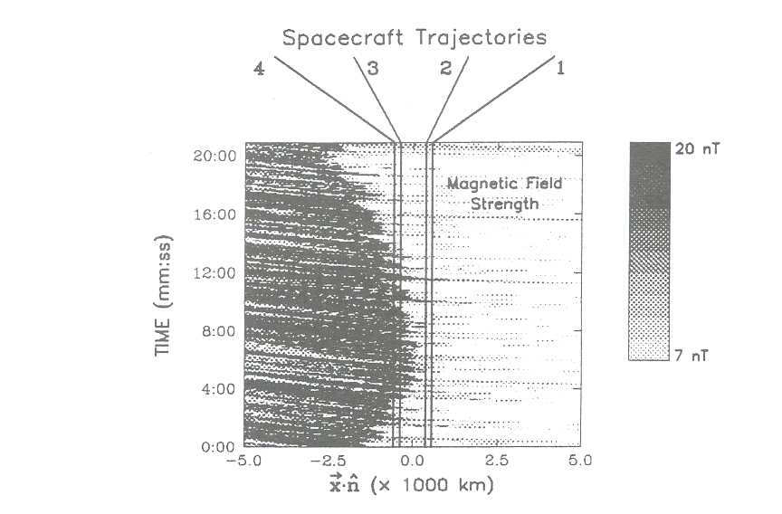
This mode of working prompts a new way to deal with the large volumes of data that a simulation can produce. One way to extract useful data from the simulation is to use a "software instrument" which has as output a time series that mimics the time series that would be produced by a spacecraft experiment in a similar plasma situation. Crudely speaking, one takes a spacecraft and "flies" it through the simulation. One can then compare the time series with the global configuration of the simulation.
We give here a practical example of the output from a software instrument. This is intended simply to give a flavour of what might be done using this technique. A full description is presented elsewhere [6].
We have developed additional software which provides a "simulated spacecraft," that we may "fly" through our simulation. At the present, the software instruments are for the magnetic field and a particle instrument. The software for the particle instrument is configurable in terms of energy bands and acceptance angles. We have initially configured it to mimic the AMPTE-UKS ion instrument (a plasma instrument covering the energy range 10eV - 20keV). We have simulated the case where four spacecraft pass close to a quasi-parallel shock, and we have chosen parameters corresponding to a real AMPTE-UKS shock crossing. The simulated spacecraft produce output that is extremely similar to the observations of long pulsations and SLAMS (short, large magnetic structures) which are seen at the quasi-parallel shock [7]. In particular we are interested in providing some basis for the separation strategy of the Cluster spacecraft at the Earth's bow shock. Cluster is an ESA space plasma mission consisting of four identical spacecraft, due for launch in 1995. We set the spacecraft separation as two pairs separated by 940.5 km, and each pair separated by 188 km. This mixed scale length separation strategy proves to be useful.
In Figure 1 we show the temporal evolution of the simulation as a gray scale representation of the magnetic field strength over a 104 km region near the shock over a 20 minute interval. Note that the spatial profiles are plotted against the shock normal direction (θBn = 10°, θVn = 25°, MA= 7.5). Regions of field strength greater than 20 nT are black, while those less than 7 nT are white. Spacecraft trajectories are indicated by the four vertical lines (at rest with respect to the average shock frame). The shock is readily identifiable, initially located at ∼ -1300 km, passing over spacecrafts 3 and 4, and then retreating to ∼ -2500 km at the end of the simulation. Interestingly, although this large scale "undulation" of the shock is dramatic, closer inspection reveals that the shock actually consists of convecting individual structures. Although it is difficult to tell on this rather long time scale, there is a change in the convection speed of the structures from the upstream to the downstream region. Several of these structures were formed quite far upstream of the shock.
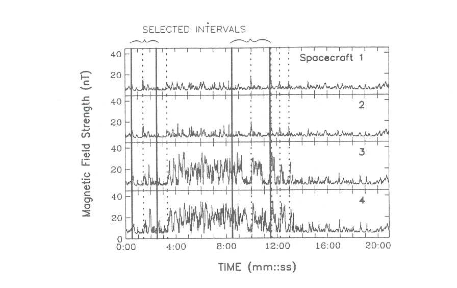
Figure 2 displays the magnetic field measured by each spacecraft as a function of time for the time interval used in Figure 1. The passage of the shock over spacecraft 3 and 4 from ∼ 3:30 to ∼ 12:30 is clearly evident. There are several structures seen by spacecraft 1 and 2 which can be associated with events seen by spacecrafts 3 and 4. Since the separation between the spacecraft pairs is 940.5 km, the solar wind will take 2.5 seconds to convect passed all four spacecraft. Hence, on the time scale shown, these structures should be roughly coincident, e.g. 1:30, 3:25, 10:00, and 11:30, the latter two being the most prominent. Spacecraft 1 and 2 did not see the pulsation of the shock while continuously monitoring the upstream solar wind conditions revealing that there were no sudden solar wind changes. Since we know that this event is a quasi-parallel shock crossing, we can conclude that the transition scale from upstream to downstream is comparable to the separation between spacecrafts 2 and 3, which is about 750 km. Note that the last two statements would not be deduced from the time series if all four spacecraft were too close together. In fact, the separation strategy chosen is quite revealing.
Currently, we are studying another type of collisionless shock, the quasi-perpendicular shock. At this type of shock the magnetic field is nearly perpendicular to the shock normal, and the stucture is very different to the quasi-parallel shock. There is little turbulence generated upstream of the shock, and the profile is more laminar, and more like a fluid shock. In ths type of shock the role of the electrons can become more important, especially for the development of whistler waves. In order to simulate this kind of shock we cannot use the hybrid method (as above), since that basically ignores any kinetic effects of the electrons. Therefore, we are using an simulation which follows both ions and electrons kinetically. We use an implicit method for the field solution which allows us to safely ignore the very high frequency phenomenae associated with the electrons (e.g., the electron plasma frequency). We can then follow the 'shock over ion length and time scales, which is absolutely vital, since it is the ion kinetic behaviour which controls the overall, average, shock structure. A further level of complexity is added by the fact that the simulations have to be carried out in two dimensions, to resolve the shock propagation direction, as well as the direction of any unstable waves. This work is being undertaken in collaboration with D. Krauss-Varban (University of California at San Diego).
Our preliminary simulations have begun to reveal the details of upstream whistler waves, generated by particles heated at the shock. The role of these waves in determining the microstructure of the shock, and in the collisionless process by which the electrons are heated, is currently under study.
This work was supported by SERC (UK) grant GR/H09454 and by the Commission of the European Community under contract SCI* 0468-M (EDB). DB holds an SERC Advanced Fellowship. Computations were carried out at the Atlas Centre (RAL, UK).
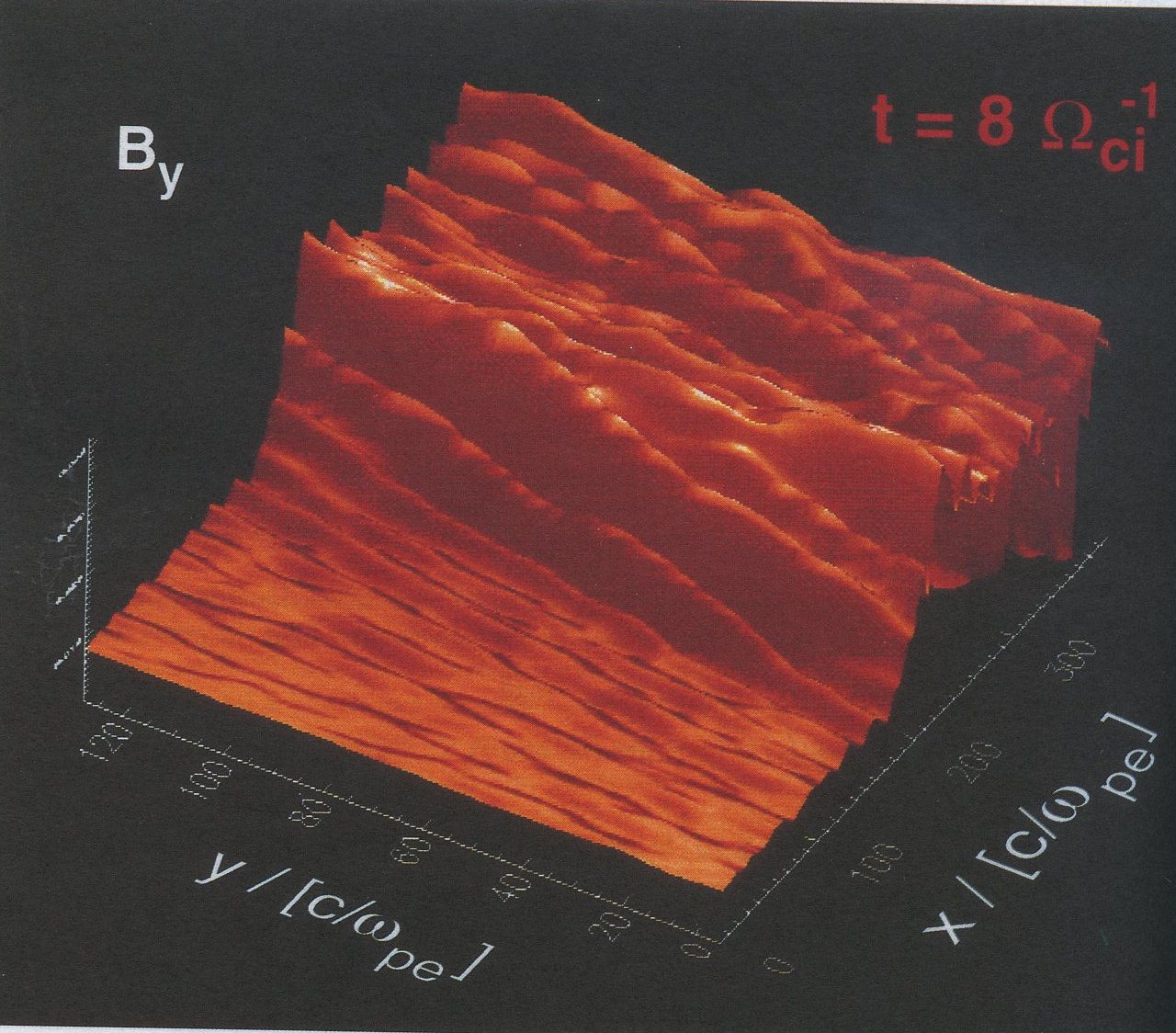
1. Singh, H. P., and K. L. Chan, A&A, 279, 107, 1993.
2. Singh, H. P., I. W. Roxburgh, and K. L. Chan, Three-dimensional simulation of penetrative convection: penetration above a convective zone. A&A, in press, 1994
3. Burgess, D., Geophys. Res. Lett., 16, 345, 1989.
4. Giacalone, J., D. Burgess, S. J. Schwartz, and D. C. Ellison, Geophys. Res. Lett., 19, 433, 1992.
5. Giacalone, J., D. Burgess, S. J. Schwartz, and D. C. Ellison, Astrophys. J., 402, 550, 1993.
6. Giacalone, J., S. J. Schwartz, D. Burgess, Artificial spacecraft in hybrid simulations of the quasi-parallel Earth's bow shock: Analysis of time series versus spatial profiles and a separation strategy for CLUSTER, Ann. Geophys, submitted, 1993.
7. Schwartz, S. J., D. Burgess, W. P. Wilkinson, R. L. Kessel, M. Dunlop and H. Liihr, J. Geophys. Res., 97, 4209, 1992.
Calculations have been performed on excitation rates and spectral transitions for small molecules of astronomical interest. Particular attention has focused on the molecules H+ 3 and water. Emissions due to H+ 3 have been observed in the atmospheres of the planets Jupiter, Uranus and Saturn, and tentatively in supernova 1987a. These spectra give extensive information on the temperature, chemical composition, time variation etc of the ionospheres of these planets. All this analyse relies on calculated transition intensities. Extensive line lists and associated intensities have been computed and are being used by several groups to model atmospheres containing H+ 3.
Vibrational excitation rates have been calculated for electron collisions with H+ 3 and HeH+ using the UK molecular R-matrix code. The rates were found to be significantly different from previous, cruder, estimates. The increased H+ 3 excitation rate is an important parameter in models which attempt to form molecular hydrogen in the absence of grains.
In cool, oxygen rich stars such M-dwarfs, water is expected to be the dominant absorber of radiation in the infra red. Calculations of all the possible infra red transitions of hot (3000+ K) water are being undertaken to aid the modelling of cool star atmosphere. So far 107 transitions have been computed. The figure compares our (by molecule) absorption spectrum of 3000K water (inset) with the spectrum of the star VB10 observed by HRA Jones and AJ Longmore. The agreement is encouraging although our data needs to be extended and included in a full stellar model before a complete comparison can be made.
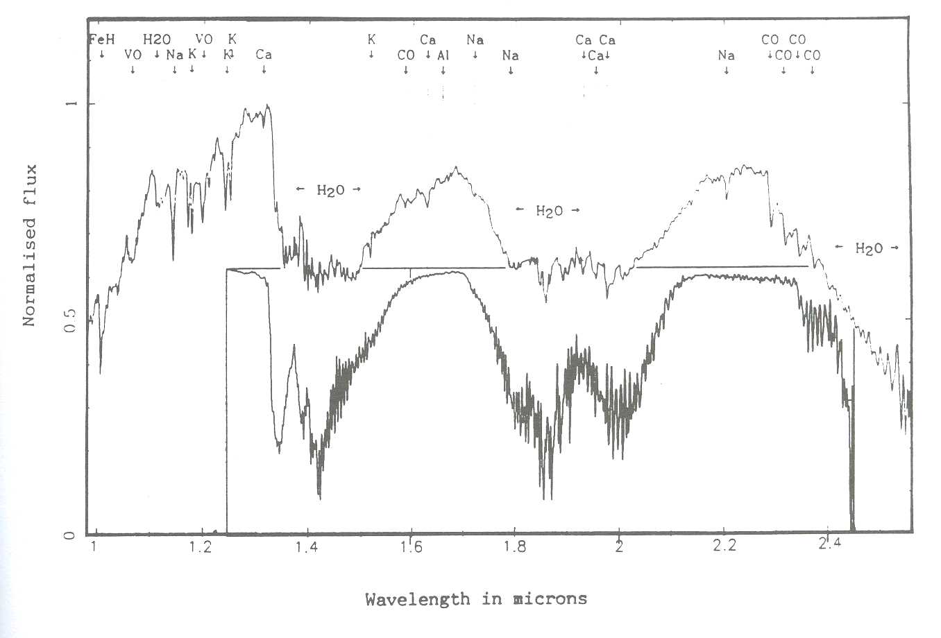
A group in the Department of Physics & Astronomy of The University of Wales College of Cardiff, lead by Alistair Nelson and Anthony Whitworth, have been working on a project to study how stars form, funded by the Science and Engineering Research Council.
The work involves the simulation of self-gravitating interstellar gas on the CRAY supercomputer at the Rutherford Laboratory in Oxfordshire, with the results being brought back to Cardiff for graphical display and analysis in the form of computer movies. As well as using the most up-to-date computing equipment the project has employed some of the most modern numerical techniques for modelling gravitation and gas dynamics. These have enabled the computer to follow the gas through an increase in density by a factor of ten thousand million and have reached the point where the protostar is a tiny spinning disc, emitting radiation in the infra-red. This is the first time that such calculations have been carried out on a computer, and represents a quantum leap in the theoretical modelling of star formation.
Stars are forming all the time from diffuse clouds of interstellar gas in our Galaxy, with the material being pulled together by its self gravity. However, despite many years of international effort, astrophysicists are still far from understanding how this happens in detail. These calculations will go a long way to rectifying that situation, and should lead eventually to a much more complete understanding of the process.
The original aim of this project was to develop and implement a numerical code which could treat the self-gravitating hydrodynamics of supersonic interstellar gas clouds, and then to simulate and evaluate different scenarios for protostellar collapse. The code we have developed combines Smoothed Particle Hydrodynamics (SPH; Lucy 1977, and Gingold & Monaghan 1977) and Tree-code Gravity (TCG; Hernquist 1987).
The main purpose of the original grant was to fund an RAIA, and to provide computing resources on the CRAY XMP at RAL during the period 89/91. Dr. Helen Pongracic took up the RAIA post in January 1989, having completed a Ph.D. with Professor J.J. Monaghan at Monash University. She brought with her considerable expertise in SPH, and together with Dr. J.R. Davies (then a PG student of AHN) wrote and tested the combined SPH and TCG code based on a FORTRAN version of TCG obtained from Lars Hemquist. We argued in our original application that the combination of SPH and TCG would yield a code which is (a) fully Lagrangian, (b) totally devoid of symmetry assumptions, and (c) able to follow very large density increases. These features are essential if one is to model the complex structures and large density contrasts involved in star formation. In the event the performance of the code has significantly exceeded our expectations. It has given good physical modelling up to density contrasts of 1010, simulating the formation of rotating, accreting protostellar discs from cloud material starting at interstellar densities. Dr. Pongracic carried out the first interstellar cloud/cloud collision runs to produce protostars (Pongracic et. al. 1992), and continued with the application of the code during 91/92 supported by funds from the Leverhulme Foundation.
The purpose of the grant of which this is the final report (ref GR/H 37341 ), was to continue the simulations on the CRAY at RAL during 91/92, specifically to explore the cloud/cloud collision parameter space, and to investigate the formation of binaries. In the event, a second small grant of CRAY time (ref GR/H 86240) was also awarded due to an underprovision against the requested resources, and to the increase in the, resources available at RA after the arrival of the YMP.
During 91/92 Dr. Simon Chapman (then a PG student of APW) made significant contributions to the development of the code, including further work on vectorisation and the development of equilibrium isothermal models for the interstellar clouds - in contrast to the non-equilibrium, uniform density clouds used previously. Dr. Chapman was able to make very good use of early access to the YMP in the summer of '92 to perform calculations involving larger mass clouds with more SPH particles.
Some of the work on binary formation during the grant period was reported in an article in Nature (Chapman et. al 1992). The main conclusion of this work was that binaries can form during the off-axis collision of interstellar clouds, either by a process of thermal fragmentation followed by subsequent partial merging of the fragments, or by a process closer to rotational fission in which the fragmentation of a spinning central object is induced by accretion. Examples of these are shown in Figures 1 and 2. In Figure 1 two uniform clouds collide; in frame (c) the fragmentation caused by the combination of gravity and thermal instability can be seen, leading aver merging to a binary seen in close-up in frame (d) [the time sequence is a,b,c,d and the x-scale of the boxes is 7 × 10⁵ A.U., 7 × 10⁵ A.U., 7 × 10⁴ A. U., and 104 A. U. respectively]. On the other hand Figure 2 shows the collision of two equilibrium clouds in hydrostatic balance. This time a single central rotating object is formed, which subsequently fragments in to four separate masses in frame (d) [here the x-scales are 8 x 10⁵A.u., 1.6 × 10⁵AU., 2 × 10⁴A.U., and 2 × 10⁴A U.].
The calculations in Figs. 1 and 2 involve the collision of clouds with 75 M0 of material each, leading to the formation of a few protostellar objects with masses in the range 2-40 M0 each. By contrast Figure 3 shows the final result of the collision of two clouds of 750 M0, carried out by Dr. Chapman on the YMP. Here the thermal fragmentation process leads to the formation of at least 16 protostellar objects with masses in a similar range. Note that each of these objects is a centrifugally supported, accreting protostellar disc. In the original SERC application to fund the Star Formation project at Cardiff, we predicted that the combination of SPH and TCG would enable the simulation of the formation of a small cluster of stars. This result, and others like it, vindicate that prediction. It also turns out that some cusp-like features which we observed in the low cloud mass calculations show up as filamentary features connecting the several protostars in the case of the high mass cloud collisions.
These calculations have demonstrated that it is possible to simulate the formation of multiple protostars, starting from realistic initial conditions, and that the dimensions of the systems formed are similar to that of observed putative protostellar discs (Saudel et al. 1991, and Wooten, 1989), and pre-main sequence multiple systems (Zinnecker, 1988, and Clarke, 1992). The ubiquity of the fragmentation processes suggest that binary and multiple star systems will be the rule rather than the exception.
Further work on simulating Star Formation is continuing in Cardiff under the leadership of Dr. Whitworth, while Dr. Pongracic has returned to Australia, and is continuing to collaborate with the Cardiff group on the simulation of Star Formation by large scale shocks.
Chapman, S.C., Pongracic, H., Disney, M.J., Nelson, A.H., Turner, J., & Whitworth, A.P., Nature, 359, 207-210, 1992.
Clarke, C.J. Nature, 357, 197-198, 1992.
Gingold R. & Monaghan J., MNRAS 181, 375, 1977. Hernquist L., Ap J Suppl Ser. 64, 715, 1987.
Lucy L., AJ. 82, 1013, 1977.
Pongracic, H., Chapman, S.C., Davies, J.R., Disney, M.J., Nelson, A.H., & Whitworth, A.P., MNRAS, 256, 291-299, 1992.
Sandell, G. et. al. Ap.J, 376, L17-20, 1991. Wooten, A.,Ap .. J., 337, 858-864, 1989.
Zinnecker, H. in Low Mass Star Formation & Pre-Main Sequence Objects (ed. Reipurth, B.) 447-469 (ESO, Garching, 1989)
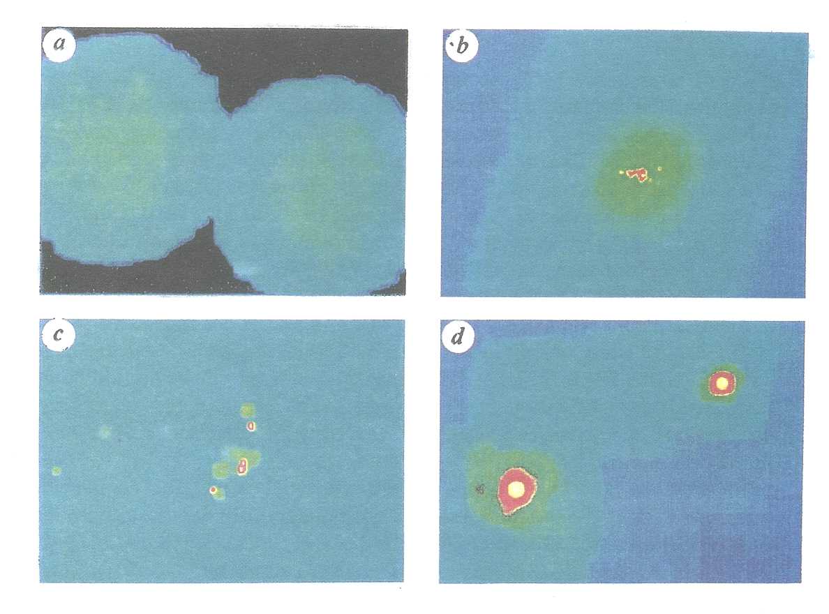
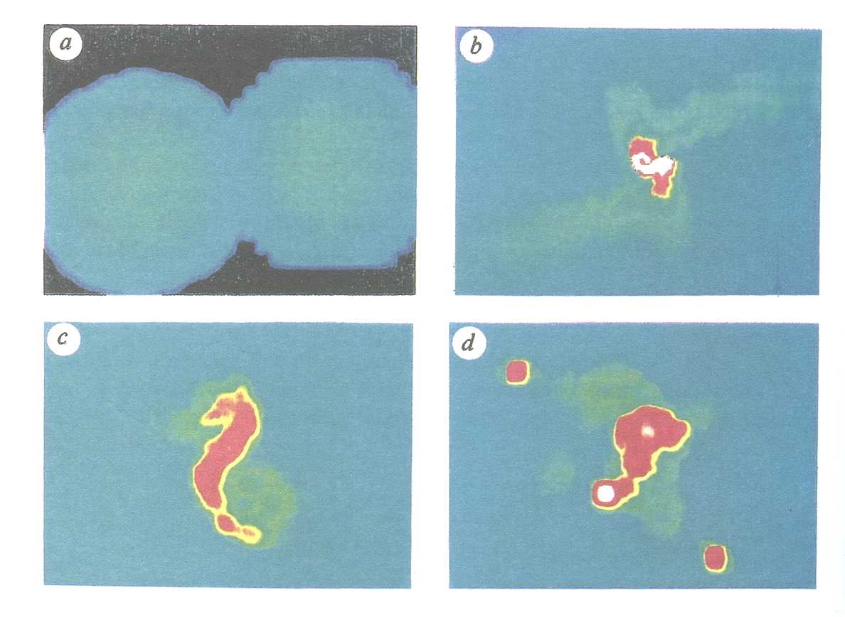
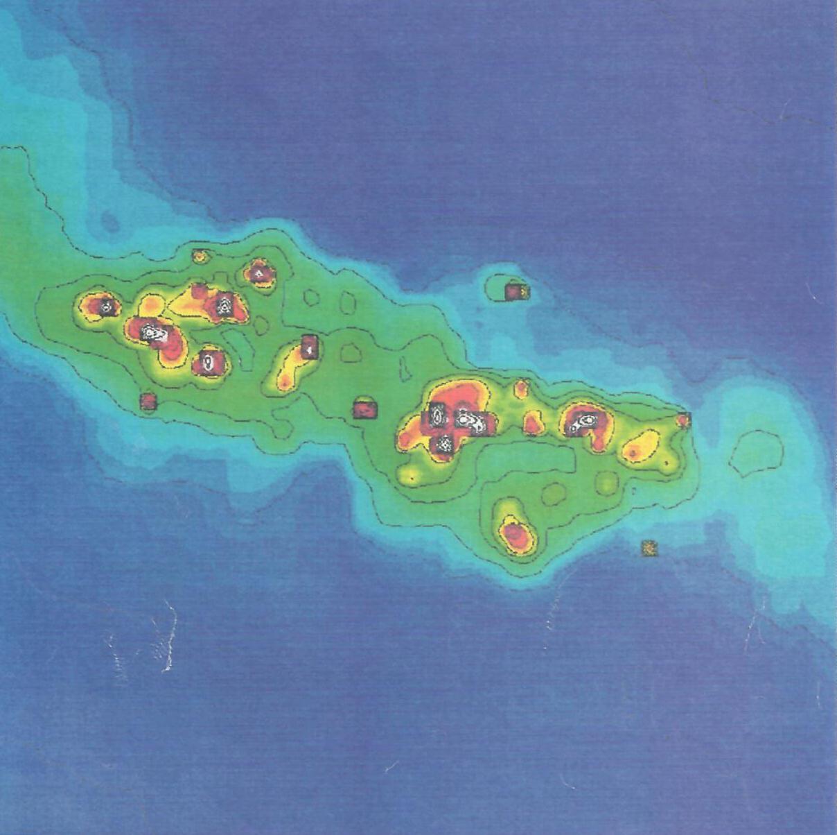
The upper part of the HR diagram contains a number of post-main sequence massive, luminous stars: the Luminous Blue Variables (LBVs); extreme Of and Ofpe/WN9 stars; P Cygni-type stars; and the Wolf-Rayet (WR) stars. These stars are key objects for our understanding of the evolution of the most massive stars formed in galaxies yet their evolutionary connections are not understood. In particular, Wolf-Rayet (WR) stars are believed to be the evolved descendants of massive O stars which have undergone extensive mass loss, have shed their hydrogen envelope and exposed the products of core CNO-burning (WN) and He-burning (WC, WO).
The difficulty in developing codes suitable for modelling WR spectra results from: (1) The wind ionization in WR atmospheres is determined primarily by the intense radiation field from the hot stellar core rather than the local electron temperature thus requiring non-LTE; (2) The usual plane-parallel stellar atmosphere are not applicable since WR stars have extended atmospheres; (3) The large velocity gradiant found in WR atmospheres means that the transfer equation is not readily solvable in the observers frame thus requiring solution in the comoving frame (CMF). It is only in the past few years that codes have become available which are able to correctly model line and continuum formation in WR atmospheres. Such codes have been developed independently by D.J. Hillier (1987,1990) and by W. Schmutz and W.-R. Hamann (Hamann and Schmutz, 1987). In our model atmosphere code the transfer equation for multilevel atoms is solved in the CMF, under the simplifying assumptions of time independence, spherical symmetry and homogeneity, subject to the constraints of statistical and radiative equilibrium using the technique developed by Hillier. The WR model atmosphere currently comprises model atoms of hydrogen, helium, carbon, nitrogen, oxygen and silicon and a prescribed mass-loss rate, luminosity and velocity law. Typical Cray-YMP job requirements to arrive at a converged model are approximately 900-3600s processor time and 4-l0Mw memory.
Detailed analyses have been performed for 24 Galactic WN stars (Crowther et al. 1993a). We find that not all massive WR stars are necessarily post-LBV objects - we find that some (the 'WNL+abs' stars) have directly evolved from Of stars. Carbon and nitrogen abundances of the Galactic WN stars are generally found to be consistent with predictions of evolutionary models (e.g. Maeder 1990). Examples of theoretical profile comparisons with observation are shown in Fig.l for WR40 (WN8).
The Ofpe/WN9 stars, found exclusively in the LMC, apparently show a composite spectrum of high excitation Of and low excitation WN features. We have conducted a study of a subset of these stars (Crowther et al. 1993b) and find them to be located in a thin temperature strip in the H-R diagram slightly cooler than Galactic WNL stars. Chemically, these are in reasonable agreement with the latest evolutionary predictions for post-RSG stars having just entered the WN phase at low metallicity (Schaerer et al 1993).
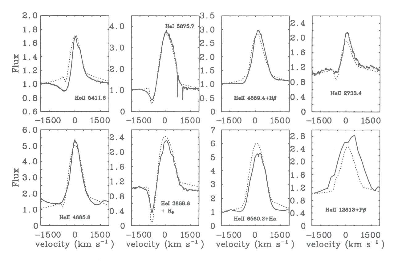
Finally, quantitative studies of the LBV AG Carina, and the LBV candidate He 3- 519, have been made (Smith et al. 1993), with both objects found to be evolved massive stars near the observed upper luminosity /stability limit in the HR diagram. Both stars are found to be spectrally and chemically cool members of the WN sequence at minimum and so can be thought of as unstable W-R stars.
Use of the RAL Cray-XMP and, more recently, Cray-YMP supercomputers have proved to be crucial for our studies of massive star evolution. This programme is being extended to detailed studies of WR stars in the Magellanic Clouds; a broader sample of LBVs P Cygni stars and extreme Of stars; and modifications to the non-LTE codes for which the YMP will continue to be essential.
Crowther, P.A., Smith, L.J. & Hillier, D.J., 1993a, in: Evolution of Massive Stars: A Confrontation between Theory and Observations, eds. D. Vanbeveren, W. Van Rensbergen & C. de Loore, Space Sci. Rev., in press.
Crowther, P.A., Hillier, D.J. & Smith, L.J., 1993b, A&A, submitted.
Hamann, W-R. & Schmutz, W., 1987. A&A, 174, 173. Hillier, D.J., 1987. ApJ Suppl., 63, 94 7.
Hillier, D.J., 1990. A&A, 231, 116.
Maeder, A., 1990. A&A Suppl., 84, 139.
Schaerer, D., Meynet, G., Maeder, A. & Schaller, G., 1993. A&A Suppl., 98, 523.
Smith, L.J., Crowther, P.A. & Prinja, R.K., 1993. A&A, in press.
Crowther, P.A., Smith, L.J. & Hillier, D.J., 1993, "Tailored analyses of 24 Galactic WN stars", in: Evolution of Massive Stars: A Confrontation between Theory and Observations, eds. D. Vanbeveren, W. Van Rensbergen & C. de Loore, Space Sci. Rev., in press.
Crowther, P.A., 1993, PhD Thesis, "Model Atmosphere Studies of Wolf-Rayet Stars", University of London.
Crowther, P.A., Hillier, D.J. & Smith, L.J., 1993, "Fundamental Parameters of WolfRayet Stars I. Ofpe/WN9 stars", A&A, submitted.
Smith, L.J., Crowther, P.A. & Prinja, R.K., 1993, "A study of the Luminous Blue Variable candidate He 3-519 and its surrounding nebula", A&A, in press.
The group led by Dr Janet Drew at Oxford, Astrophysics has been using the Cray YMP to investigate the phenomena of mass-loss in certain types of hot stellar objects. In particular this has focused on a type of binary star called a cataclysmic variable where the two orbiting stars are interacting with each other. These systems consist of a very compact white dwarf star which is about the size of the Earth but still about as massive as the Sun and another more normal star similar but less luminous that the Sun. These stars are in a very close binary which has an orbital period of only a few hours. The gravitational field of the white dwarf is so strong that it pulls matter from the outer layers of the other star. Since the stars are in orbit around each other the stream of matter interacts with itself to form a disc of material around the white dwarf.
As the matter in the disc spirals slowly towards the surface of the white dwarf the release of gravitational potential energy heats the gas up to tens of thousands of degrees. This makes the disc the most luminous part of the system in the UV and optical wavebands. In certain systems instabilities in the mass transfer mechanism cause the accretion rate to increase rapidly for a few days every month or so, causing the system to brighten by about a factor of a hundred; hence the name: cataclysmic variable.
It is during these periods of high mass transfer that another phenomenon is noted - that of significant mass-loss from the system. This was recognised spectroscopically by the presence of a strong blueshifted absorption component in UV resonance lines observed via satellites. For systems orientated such that we see the disc more-or-less face on the wind-formed absorption line, as seen against the strong background of UV continuum light from the disc, is Doppler shifted blueward since the gas is flowing towards us. The maximum velocity deduced from the spectral line profiles is about 5000 km s-1 which is similar to the escape speed from the white dwarf so it is thought that the wind originates from at or near the centre of the disc. However, the mechanism which drives these winds and how it affects the evolution of these systems are not known. Other, less well understood types of object are also thought to contain winds which originate from accretion discs such as stars which are still in the process of forming and the centres of peculiar types of active galaxy.
In order to deduce the total mass-loss rate in these outflows we must first determine the abundance of the various ionization stages that form the observable lines, i.e. C IV λ1549Å, N V λ1240Å and Si IV λ1397Å. Since we cannot currently observe the resonance transitions of all the possible ions of a particular element that may be present in the wind we must resort to calculations of the ionization structure. This will also be of use when attempting to determine the detailed velocity structure of the winds from the line profiles.
To study the ionization state of these optically thick winds we have developed a radiative transfer code by Drew (Drew & Verbunt 1985, Drew 1989 Hoare & Drew 1993), to include an accurate treatment of the continuum radiation field using approximate lambda operator techniques (see Rybicki 1991). We solve the equations of statistical equilibrium self-consistently with the radiation field for 16 levels of H I and He II, 8 levels of He I and the ground and important excited states of the ions of the eight next most astrophysically abundant elements. The physical processes taken into account are radiative photo-ionization, recombination and bound-bound transitions and the corresponding collisional processes. Transfer in the lines was treated using the Sobolev approximation.
To make the problem tractable we assume spherical symmetry although some account of the axisymmetric nature of the continuum radiation field from the accretion disc is made at optically thin frequencies. The density structure is specified by choosing a total mass-loss rate and a velocity law for the wind which is known to approximately match the observed line profiles. We also use the constraint of radiative equilibrium to solve for the temperature structure of the wind. Typical models with over 100 depth points required about 50 iterations of the radiation field/level population calculation in order to get the relative corrections in the He II ground state population to less than 1%. This usually took about 1 hour CPU time on the CRAY YMP.
The input radiation field at the base of the wind includes an accretion disc component with the spectrum predicted for a steady accretion rate and with each part of the disc radiating as a blackbody at the appropriate temperature (e.g. Pringle 1981). Previous models had also usually included a hot (TBL ≈ 300 000 K), luminous boundary layer since this is predicted to occur between the disk and the white dwarf unless it is rotating close to break up (Pringle 1977). This component arises as the rapidly rotating material at the inner edge of the accretion disc shears onto the surface of the white dwarf. It should be observable using soft X-ray satellites, and although there have been some claims that this has indeed been seen there were also increasing numbers of observations which appeared not to detect the predicted level of emission. We therefore calculated photo-ionization models with much cooler boundary layers than predicted theoretically and ones with no boundary layer at all and for a range of different wind mass-loss rates. The radially averaged concentrations of the ions which form the observable lines were then compared to those deduced from synthesizing real spectra.
We found that a good match to the observed ion concentration in the winds could be obtained by invoking either a cooler boundary layer than hitherto thought (⪝ 100 000 K) or having no boundary layer at all but with a slightly higher accretion rate in the disc which results in a hotter inner disc temperature. These results would be consistent with the white dwarf star having been spun up to close to its break-up velocity due to sustained accretion of high angular momentum material. An important consequence of using cooler radiation fields is that the ionization fractions of the observable ions are higher which means that the derived total wind mass loss rates are lower. In our models they are now only a few percent of the mass accretion rate which means that, unlike previous studies, the pressure of radiation from the disc now has enough momentum to drive these winds. More realistic 2D and 3D calculations with nonspherical outflow geometries will be needed before we can be confident that we fully understand the dynamics of these winds, but studies of the cataclysmic variable systems are a vital step on the road to increasing our knowledge of accretion disc winds in general.
Drew, J.E. and Verbunt, F. 1985, MNRAS, 213, 191 Drew, J. E. 1989, ApJS, 71, 267.
Hoare, M. G., & Drew, J. E., 1993, MNRAS, 260, 647. Pringle, J.E. 1977, MNRAS, 178,195
Pringle, J.E. 1981, ARA&A, 19, 137
Rybicki, G. B., 1991. in Stellar Atmospheres: Beyond Classical Models, eds. L. Crivellari, I.
Hubeny, D. G. Hummer, Kluwer, Dordrecht, p. 1.
M. G. Hoare & J. E. Drew, The Ionization State of the Winds from Cataclysmic Variables Without Classical Boundary Layers Monthly Notices of the Royal Astronomical Society 260 (1993) 647