

Appendices
- A: Heat, work, the conservation of energy, and the First Law of Thermodynamics
- B: The Einstein model and the Kelvin temperature
- C: The quantum shuffling game for indistinguishable quanta
- D: Photographs of pucks distributed between two halves of a surface
List of books, films and film loops, slides and apparatus
Index
Appendices
A: Heat, work, the conservation of energy, and the First Law of Thermodynamics
This Appendix was written mainly to clear our own minds. It may be of use to teachers who wish to have a summary of some of these ideas, and of the difficulties involved in them. Most of the ideas will appear only in treatments of thermodynamics that go beyond the requirements of a sixth form course. The ideas outlined below are subtle, hard to grasp, and need play no part in teaching at sixth form level other than in indicating potential confusions to be avoided.
At the microscopic or atomic level, if the conservation of energy holds good, the sum total of the energies of any collection of atoms remains constant, however this energy may be redistributed among them. Of course, all atoms taking part in the energy transactions must be counted in.
At the macroscopic level, for matter in bulk, a parallel - but not identical - principle can be found; the First Law of Thermodynamics. Such difference as there is between the First Law and the energy conservation principle turns on the possibility of making up a macroscopic thermodynamics which does not depend on a microscopic interpretation. Macroscopic thermodynamics depends only on the results of macroscopic experiments. Reasons can be given on a microscopic picture why these macroscopic experiments turn out as they do. The reasons are not necessary to the development of macroscopic thermodynamics, but they illuminate it. Such reasons appear below.
One central concept of macroscopic thermodynamics is that of the parameter of a system. On a microscopic view, a system is a collection of very many atoms interacting with each other. If there are only a few atoms, there is little more to say. But if there are very many, say 1023, a new simplicity emerges. The behaviour of a collection of many atoms will have very stable average properties. In a gas, for example, the number and the velocity of atoms hitting a wall will both have steady average values. At the macroscopic level, as a result, a steady pressure exists, and can be picked out as one of the parameters of this system.
Macroscopically, the existence of a measurable, stable parameter pressure is just a fact of experiment, and might still be true were the microscopic gloss quite wrong (if, say, matter were continuous rather than atomic). Similar remarks can be made about other macroscopic thermodynamic ideas, but we shall not labour the point. Note, however, that if the atomic gloss is right, macroscopic thermodynamics only works for large enough lumps of matter. Two or three molecules in a box have nothing that can decently be called a pressure.
Similar remarks apply to the state of a macroscopic system. Microscopically, the large numbers of atoms involved ensure that the average overall behaviour of the collection will stay much the same, despite an enormous variety of motions and energy interchanges among the atoms. Two boxes of the same gas, both with 1023 molecules and the same total energy will inevitably behave in a quite similar way, even though their detailed atomic motions are utterly dissimilar. The powerful effects of statistical averaging ensure that a large enough system will have a definite state fixed by only a few parameters (pressure, temperature, and density, for example, each of which is a statistical average). Again, a collection of only a few molecules has no such state in the thermodynamic sense, for the actual individual motions of the molecules are very important in deciding its future behaviour, and no simple stable average behaviour emerges.
The above remarks serve to introduce the distinction between the conservation of the energy of a collection of many molecules, and the First Law of Thermodynamics applied to such a system. Conservation of energy says that there will exist a fixed total energy. The First Law says that there exists a quantity U, the internal energy, that will be the same for a system whenever its (few) thermodynamic parameters are the same.
For a gas sealed off in a rigid, insulated box, conservation of energy ensures that there will be a fixed total energy. But the First Law adds that the internal energy will have the same value whenever the gas has the same pressure, temperature, and density, that is, when it is in the same state.
Briefly, the internal energy U is a function of state. For only a few molecules, this makes no sense, though energy conservation still holds. There now exists no simple average behaviour and the total energy, though it has a definite value, cannot be simply related to a few parameters that describe any such collection as a whole, for every such small collection behaves quite differently from every other one. Crudely, the First Law equals energy conservation plus the existence of the statistical equilibrium behaviour of large numbers of atoms. Energy conservation is obeyed, so far as we know, by all-collections of atoms. The First Law is only obeyed, and at that only on average, by collections of very many atoms.
Work, the product of force and distance, can best be regarded as a means of energy transfer. On a classical, non-quantum, atomic picture, work is essentially the only means of energy transfer between atoms. The classical atoms exert forces on one another and exchange energy smoothly as they move relative to one another. On a quantum picture, energy changes are not smooth and work is not such a useful concept. On this picture, the atoms of a system have access to a number of energy levels, and all changes involve either the passage of atoms from one level to another. or the alteration of the energies of the levels, or both. Transitions between the energy levels become the primitive concept that replaces the idea of work.
At the macroscopic level, work is, as usual, the product of a force and distance, or, in general, of a pair of quantities analogous to these two. But here the forces are statistical average quantities over many atoms. If the number of atoms were small, the macroscopic work would have to be replaced classically by a sum of force-multiplied-by-distance calculations for individual atoms or, on a quantum picture, by a sum over changes in the quantized energy levels of a collection of atoms.
Heat, unlike work, is a wholly macroscopic concept. There is no meaning whatever to be attached to the heat exchanged by a pair of atoms. We may interpret heat as the transfer of energy between collections of large numbers of atoms as they spontaneously reach a statistical equilibrium distribution of energy. This attainment of statistical equilibrium is observed on the large scale as the attainment of thermal equilibrium by a system which initially has temperature differences between parts of itself. Thus heat flow only occurs from hot bodies to cold ones. An energy transfer not of this sort is not heat flow.
This use of the word heat is in part at odds with its everyday use. We usually speak of the heat stored in a storage heater, for instance. A thermodynamicist would regard the storage heater as having been given extra internal energy, and would point out that the internal energy had been raised by working electrically, not by heating the radiator. He would agree with the rest of us, however, that there is a flow of heat from the radiator to the room it is intended to warm, for this energy flow comes about as the system room-plus-heater moves towards thermal equilibrium.
Macroscopically, heat can be given meaning independently of any microscopic interpretation. The variation of the internal energy of a system with its pressure, density, and other parameters, can be mapped out by adding or removing energy by way of work alone. Finding that other changes can occur, such as those in which a gas cools without contracting, in which the internal energy change is no longer equal to the work, the heat flow is defined as the difference between them. But this viewpoint, being purely macroscopic, conceals the feature that heat flow, unlike total energy, is a concept with only a macroscopic meaning.
In short, heat flow occurs when systems move towards thermal equilibrium, and thermal equilibrium is a wholly statistical phenomenon, of systems containing large numbers of atoms. It has no counterpart in collections of only a few atoms.
Except in the usage of ordinary language, and by implication in the usage heat capacity, heat is not the same as the energy content of a body. Nor is it an identifiable part of this energy content. The internal energy of a body may change by way of work, or by way of heat flow, or by way of both. Heat is a bird of passage; a way of changing the internal energy of things, not a quantity they can contain.
We repeat that this subtle usage is presented here for information. There is no merit in pressing it upon students before they can understand that there is a case for modifying the ordinary usage. Nor is the thermodynamic usage correct and the ordinary one wrong. The thermodynamic usage is convenient and consistent for certain purposes for which the ordinary usage is not.
It may be advisable not to refer to processes such as the warming up of a body by the flow of electricity or by friction as cases of work being turned into heat. In such cases, energy is exchanged by way of work and the internal energy of the body rises and it becomes warmer. The energy has been spread out (or shared out) amongst many atoms or molecules, and it is this which makes the process irreversible. So one may say that the energy, once stored in a battery, or in a moving mass, or in some form of potential energy, has been spread among a large number of atoms.
While it may be good to encourage students to speak in such a manner, it would be premature to insist that they do so.
B: The Einstein model and the Kelvin temperature
The Einstein model makes the approximation that a monatomic solid can be represented by a collection of harmonic oscillators, sufficiently independent of one another for the energy levels of each oscillator to be identical with those of an isolated oscillator, but weakly coupled so that the oscillators share energy with one another.
The energy levels of an isolated oscillator are equally spaced, at intervals ε = hf, where f is the classical oscillation frequency, and h is the Planck constant. The lowest level has the zero point energy ½hf, but as the oscillator cannot have less than this energy, the energy of the lowest level can be treated as if it were zero. If all oscillators are alike, they thus exchange energy only in lumps or quanta of energy ε.
The number of ways of arranging quanta of energy on the oscillators may therefore be counted, as in figures 69 and 70, by counting the number of ways of placing marks differently in boxes.
The calculation of W for an Einstein solid
Figure 94 shows a general way of noting down any one arrangement of q quanta amongst N oscillators. The circles stand for oscillators, listed in some definite order. The symbols ε stand for quanta. The energy of each oscillator is indicated by the number of ε symbols which follow it. Thus the first listed oscillator has one quantum, the second has three, the third has none, and so on. The listing carries on until all N oscillators have had their energy specified, so that N symbols o and q symbols ε have been used up.
O ε O ε ε ε O O ε ε O ε O O ε ε ε ε O ε ε O ε  etc
until N symbols O and q symbols  ε are used
Figure 94: Representation of the state of an Einstein solid.
Any list of this form, containing N oscillator symbols and q quantum symbols, will represent a possible arrangement of the quanta among the oscillators. W is the number of such lists which are different from each other.
If one has to select a list from n distinct objects, the first choice can be made in n ways, picking any one of the objects. That leaves (n-1) ways to make the second choice, one object having been selected already. Every one of the n first choices can go with every one of the (n-1) second choices, so that the first two choices can be made in n (n-1) ways. The number of ways of making all the choices is given by
n (n-1)(n-2)(n-3) ... (3)(2)(1)
which, for short, is written n! and called factorial n.
In the list of figure 94, the first place must be an oscillator symbol o. That leaves (N+q-1) symbols to play with, and the number of their rearrangements is (N+ q-1)!. But all the q quantum symbols are alike, and interchanging the symbols makes no difference to the listed arrangement (the first atom in figure 94 has one quantum whichever ε symbol is put after it, as long as only one of them is put there). There are q! ways of making these trivial rearrangements of the q quantum symbols. Similarly, after the first oscillator symbol, the remaining (N-1) oscillator symbols can be rearranged among themselves in (N-1)! ways, without making the least difference to the meaning of the list, because the particular oscillators are indicated by their place in the list sequence, not by each having an individual symbol.
Thus W, the total number of distinct rearrangements, is less than (N+q-1)! . Every one of the uninteresting, non-significant rearrangements of oscillator and quantum symbols amongst themselves can go with every rearrangement of any kind. So the number (N+q-1)! must be divided by q! and by (N-1)!. W is then given by
W = (N+q-1)! / (q!(N-1)!)
If N = 3 and q = 3, W becomes
W = 5!/(3!2!) = (5 × 4 × 3 × 2 × 1) / ( (3 × 2 × 1) (2 × 1) ) = 10
Figure 70 shows these 10 ways enumerated one by one.
If the number of quanta is increased by one, to (q+1), the term on the top in the expression for W becomes (N+q)!, which is just (N+q) times larger than it was before, since the factorial is the same list of multiplying terms with an extra term (N + q) in front.
The term q! in the lower line becomes (q+1)!, which is (q+1) times larger than before. The term (N-1)! is unaltered. Thus W is multiplied by the factor (N+q)/(q+1), if one quantum is added. Writing W* for the new number of ways,
W*/W = (N+q)/(q+1) ≈ (1+N/q) if q is much larger than one.
The internal energy and heat capacity of an Einstein solid
Introducing the expression which defines the temperature T,
kT = ε/Δ ln W,
we have, for one quantum added,
kT = ε/ln(1 +N/q)
or
1 +N/q = eε/kT.
If the total internal energy is U, comprising q quanta of energy ε, we can write U/ε in place of q. Doing so, and rearranging the equation, give,
U = 3εL/(eε/kT-1)
where 3L has been written for N, so that the internal energy is given for one mole of atoms, equivalent to 3L independent oscillators.
Putting ε = hf gives the usual expression for the internal energy of one mole of Einstein solid.
The molar heat capacity can be found by calculating dU/dT, giving the prediction, first made by Einstein, that the heat capacity should fall towards zero as T goes towards zero.
Average distribution and most probable distribution
The expression
W*/W =(1 +N/q)
obtained above, for one quantum added to the system, leads, by the argument given in Part Five of the text, to an average distribution of atoms among energy levels which is exponential, the ratio between numbers of atoms in levels of adjacent energy being (1+N/q).
It is also possible to show that this is the most probable distribution. Figure 95 is intended to represent N oscillators placed with n0 having the least possible energy; n1 having one quantum, and so on.
Figure 95
The N oscillators can be permuted among the energy levels in N! ways. But these ways ignore the fact that the n0! permutations of oscillators in the lowest level, the n1! permutations of those in the first level, and so on, are of no account, since the order in which the oscillators are listed is of no importance. Thus
w = N!/n0n1n2...
gives the number of distinct arrangements for the one distribution in which the level populations are n0, n1, n2 ...
The most popular of such distributions will be the one for which w is largest. w will be at a maximum when a small change in the distribution produces no change in w, using the general property of turning points.
A suitable change which conserves energy in the system is to demote one atom from the j-th level to the one below, the i-th level, and promote one atom to the level above the j-th, the k-th level. Thus
ni → ni + 1
nj → nj - 2
nk → nk + 1
Substituting these new values in the expression for w, we find that w is altered by the factor
ni(ni-1)/(ni+1)(nk+1) ≈ nj 2/nink (1 ≪ n)
The factor will be unity, and w will thus be unchanged and so at its maximum, when
ni/nj = nj/nk,
w is a maximum, belonging to the most probable distribution, when the populations of adjacent levels are in constant ratio, and the distribution is exponential.
This calculation, to be found in many books, often in a more difficult form, has only modest value. It can be extended to give the value of w for the most probable distribution, but this is not the same quantity as W, the total number of distinct states consistent with a given energy. It is W which is needed if one is to make calculations of the behaviour of two systems put together, and it is W which is required for the simplest statement or the basic principle of statistical mechanics, which is that the average behaviour of a large system can be found by averaging over all of the number W of its possible distinct quantum states, giving equal weight to each. (Note that because there may be more than one quantum state with the same energy, it is better to say quantum states here than energy levels.)
The distinction between W and w can be illustrated further by the example of balls partitioned between two halves of a box. The total number of rearrangements W is just 2N, if there are N balls.
If the balls are distributed with n1 in one half and n2 in the other half, this particular distribution can be realized in w = N!/n1! n2! ways. The most popular distribution is that for which n1 = n2.
The maximum value of w, wmax, is always less than the value of W, and the ratio W/wmax becomes larger, not smaller, as N increases. However, ln wmax becomes a better and better approximation to ln W as N increases, and it is this which justifies the substitution of ln wmax for ln W in many treatments of statistical mechanics, despite the lack of fundamental significance of the quantity wmax.
Temperature and level spacing
In Parts Four and Five, the Kelvin temperature of an Einstein solid was defined by means of the equation
kT = ε/ln(1+N/q).
In the only instance of heat flow considered (in the sixth film of the series of computer films, illustrated in figures 61 to 65), the energy level spacings ε in the hot and cold bodies were identical, so that the problem reduced to something analogous to the diffusion of quanta. In this example, the energy level spacing ε plays no part in the argument, and would seem not to be needed in the above expression for the temperature.
The need to include the energy level spacing can be brought out by considering a slightly more complicated example.
Consider an Einstein solid having N oscillators and q = N quanta. The ratio (1+N/q) is equal to 2. A second such solid could have the same mean energy per oscillator, but could have levels of twice the spacing. It would have q=N/2 doubled sized quanta, and the ratio (1+N/q) would be 3.
Now suppose that this second solid gave up one of its (large) quanta. W for this solid would be divided by the factor 3. But if this energy goes to the other solid, it becomes two (small) quanta. Each of these two quanta, when added to the solid containing q = N other (small) quanta, multiplies W for that solid by 2. When both are added, W is multiplied by 2 × 2 = 4.
The effect on W for the pair of solids together, which is the product of W for each alone, is to multiply it by 4/3. Thus the transfer of energy from the solid with fewer, larger quanta to the one with more, smaller quanta, leads to an increase in W overall, and will happen. The solid with the larger quanta was the hotter of the two. It is worth noting in passing that the two solids are not at the same temperature, despite the fact that they have the same mean energy per atom.
In general, we consider a pair of Einstein solids having N, and N2 oscillators; level spacings , and ε2; and numbers of quanta q1 and q2. A small energy transfer dU will represent dU/ε1, quanta added to or removed from solid 1, and dU/ε2 quanta added to or removed from solid 2. The addition of dU/ε quanta multiplies W for either solid by the factor (1 +N/q)dU/ε.
The two will be in equilibrium when these factors are equal; that is, when (taking logarithms)
ε1/ln(1+N1/q1) = ε2/ln(1+N2/q2)
The general expression for this equality reads as
ε1/Δ ln W1 = ε2/Δ ln W2
Because the quantity ε/Δ ln W is what is the same in two systems in thermal equilibrium, it is the quantity chosen for defining the temperature T using
kT = ε/Δ ln W.
Temperature and statistics
The statistical definition of the Kelvin temperature given above is fundamental and comprehensive. Any physical system for which it is possible to measure a quantity related to Δ ln W, when energy is added or removed, can be used to measure Kelvin temperatures. In principle, one could take any material and simply count the number of atoms in two quantum states different by energy ε. If this ratio were, say, 2, and the level spacing ε were 10-20 J, the temperature would be given by
T = 10-20 / k ln 2 ≈ 1 000 K.
Something very close to this is done in practice, when temperatures are measured using paramagnetic salts. For some such salts, an adequate model is to suppose that each atom has a magnetic moment μ, and that each can have its moment either parallel or anti-parallel to an applied flux density B. A moment with its direction anti-parallel to B has extra energy μB; a moment parallel to B has reduced energy -μB. The first requires energy to be taken from the remainder of atoms, leading to fewer ways, and so will be rare. The second gives energy to be shared out, leading to more ways, and so will be common. There are thus more moments parallel to the field than there are moments anti-parallel to it, and the material has a net magnetization along the field. The magnetization varies as
eμB/kT-e-μB/kT
(If kT ≫ μB - weak moments, small field, high temperature - this reduces to
(1 + μB/kT)- (1 - μB/kT) = 2μB/kT
since ex ≈ 1 + x if x is small. This last result is Curie's law: the magnetization varies as 1/T.)
A paramagnetic salt can thus be used as a thermometer, employing the net magnetization of the specimen as a means of counting proportions of atoms in two energy states.
Needless to say, an ideal gas can also be used as a means of measuring Kelvin temperatures. For example, if a gas of N particles increases its volume from V to (V+dV), a statistical argument, like that which gives the factor 2N for the increase in W when the volume doubles, says that W is multiplied by the factor [(V+dV)/V]N. that is,
d(ln W) = N ln(V+dV)/V ≈ N dV/V.
If the expansion is reversible, W does not change overall. If the expansion is also isothermal, the compensating decrease in W comes from heat Q extracted from a heat sink at temperature T, reducing W for the heat sink by an amount given by
d ln W = -Q/kT.
In treatments of thermodynamics based on ideal gas cycles, the equality of the ratios Q/T for fractionally similar, isothermal reversible changes, is offered as a way of defining T. Here we see it as a special case of counting changes of numbers of ways.
Furthermore, the pressure P of the gas can be calculated. In the isothermal, reversible change considered,
P dV+Q = 0
so that P dV= kTd ln W = NkT dV/V
where d ln W is the change either of the heat sink or of the gas. This yields
PV= NkT
which is the usual expression for the pressure of an ideal gas, here obtained from statistical considerations. We now also see why it is common to regard the Boltzmann constant k as the gas constant divided by the number of molecules, and why temperature on the ideal gas scale can be identified with the fundamental statistical Kelvin temperature.
Sources of reference for teachers
Versions of the argument for the most probable distribution appear in
- Bent, The Second law
- Sherwin, Basic concepts of physics
- Millen (ed.), Chemical energetics and the curriculum
- Gurney, Introduction to statistical mechanics
- Sources of physics teaching. Part 1
The argument for the value of W for the Einstein solid is to be found in Bent's, The Second law, Chapters 21 and 22 (which also contains a discussion of the internal energy of an Einstein solid).
The canonical ensemble is discussed in detail in a thorough but tough treatment in Reif, Statistical physics (The Berkeley Physics Course, Volume 5).
C: The quantum shuffling game for indistinguishable quanta
One of the innovations in the text is the introduction of a game in which quanta are shuffled at random between oscillators, the quanta being counters, and the oscillators being sites located in a definite pattern. The six sequences in the film Change and chance; a model of thermal equilibrium in a solid are based on this game. The purpose of this Appendix is to outline the relationship between the game and the more orthodox statistical calculations to be found in books on statistical mechanics.
The rules of the game have been chosen so that the game reaches a statistical equilibrium which is identical with the statistical equilibrium attained by indistinguishable quanta disposed at random amongst oscillators located at distinguishable sites. It is not clear at first sight how any game played with counters which are in fact distinguishable can represent the behaviour of quanta which are not.
The rules are as follows. Each site is assigned a reference number, and sites are chosen at random, using random numbers generated in such a way that no site is favoured over any other. One move of the game consists of two steps. First a site is chosen at random, and one quantum is removed from it, if it has more than zero quanta at that time. Secondly, another site is chosen at random, and the quantum just removed is placed on it.
If the site chosen has no quanta, no quantum can be picked up, and the move is reckoned to be completed. It turns out that it is very important that all such null moves be counted in in the average behaviour of the system, if the game is to reach the required equilibrium. Before discussing this matter, we shall draw attention to the difference between our game and one other, which gives the wrong result.
Another game would simply be to place q counters down at random on N sites. This could be done by choosing the sites one by one, at random, or even by sprinkling the counters from a great height. The outcome would be the binomial distribution, whose shape is suggested in figure 96.
This distribution has a maximum, which for very many counters lies at the mean, with q/N counters per site. Clearly, if there are many more counters than sites, a negligible number of sites will have no counters.
For indistinguishable quanta shared among distinguishable sites, and also for the game whose rules are explained above, the outcome is very different. As indicated in figure 97, the distribution is exponential, so that however large the number of quanta or counters, more sites have no quanta than have any other number, and the numbers of sites with numbers of quanta different by 1 bear a constant ratio to one another.
Figure 96: Binomial distribution
Figure 97: Exponential distribution
The difference arises in quite a simple manner. Consider a three-site system, with two counters. When both counters are on one site, there is no difference between the case where the counters are distinguishable, and the case where they are not, as indicated in figure 98.
Figure 98
But when the counters are spread out, with only one site having no counter, there is a difference between the two cases, as illustrated in figure 99. Because interchanging the counters between sites makes a difference when the counters are distinguishable, but makes no difference when they are not, there are twice as many ways of arranging the distinguishable counters as there are of arranging the indistinguishable counters.
The net effect is that, on average, a system with distinguishable counters spends more time in distributions in which few sites have no counters than does a system containing indistinguishable counters. This is the source of the apparently puzzling way in which the indistinguishable counters favour distributions in which many sites have no counters, and sites with few counters are always more frequent than-sites with many counters.
Figure 99
We now consider, with the aid of a special case, how a game following the rules described can imitate the behaviour of indistinguishable quanta. Figure 100 compares two possibilities for the disposition of 36 counters on 36 sites.
Figure 100
For indistinguishable quanta, figure 100 a shows a distribution which has just one way of being realized, since no interchanges of quanta make a difference. There is no less likely distribution. Figure 100b shows a distribution that can be realized in 36 ways, depending on which site has the pile of quanta. Thus the distribution shown in b is 36 times more likely than that shown in a.
The game achieves this outcome as follows. The distribution in a will vanish on the next move in 35 out of 36 cases, since only on one move out of 36 will the quantum picked up in the first half of the move happen to be put back on the site it came from, in the second part of the move.
On the other hand, the distribution in b will live much longer, provided that all the moves which hit on an empty site in an attempt to pick up a quantum are counted. A quantum will only be picked up on one move in 36, and when it is put back on the board by a random choice of site, it will go somewhere other than to the site it came from, on 35 out of 36 occasions. The net effect is that b lives just 36 times as long as a, which is what is required for indistinguishable quanta.
It is worth noting that distinguishable counters favour these two distributions quite differently. Figure 100 b can still be realized in 36 ways, but a can be realized in 36! ways, so that far from a being less likely than b, it is 35! times more likely than b. Intuitively, if 36 counters are sprinkled over 36 sites, a is not wholly implausible as the outcome, whilst the outcome in b would be a great surprise.
A full analysis shows that the rules of the quantum shuffling game achieve the proper weight on each possible distribution so as to simulate the distributions of indistinguishable quanta. Such an analysis is given in Black, P. J., Davies, P., and Ogborn, J. M. (1971) A quantum shuffling game for teaching statistical mechanics, American journal of physics, 39, 10, 1154-1159.
D: Photographs of pucks distributed between two halves of a surface
This Appendix consists of two sets of photographs, referred to in the text of Game 9.3 Simulation of the behaviour of marbles in a tray.
The first set, figure 101 a, consists of snapshots of the positions of ten pucks moving about at random on a low friction surface. A white line divides the surface into two equal areas.
The second set, figure 101 b, was made in the same way, but the number of pucks was reduced to four.
Both sets contain enough examples of the distribution of the pucks between the two halves of the surface to make it possible to calculate the mean number of pucks in one half and to study the frequency with which, for example, all the pucks happen to be in one half.
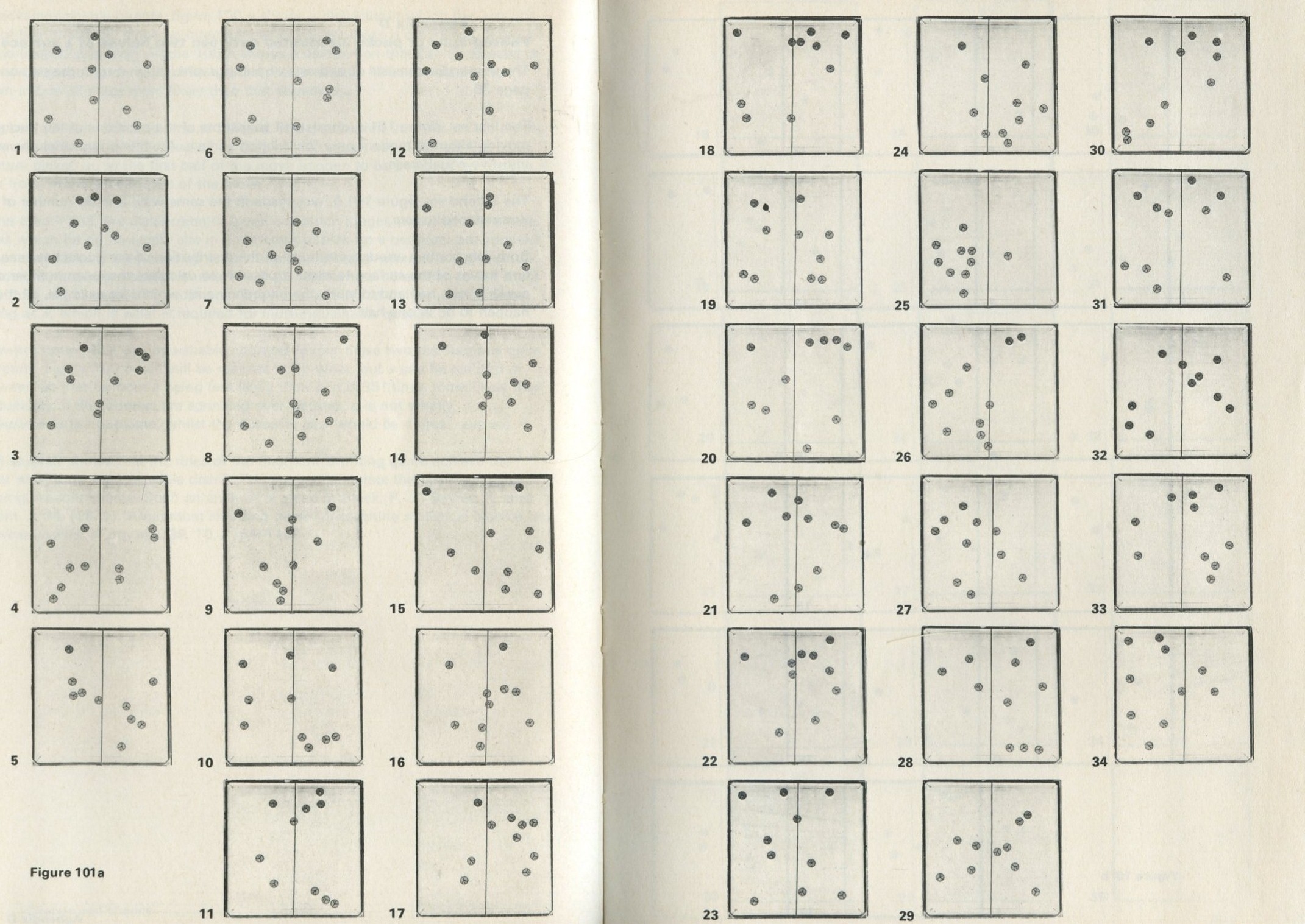
Figure 101a
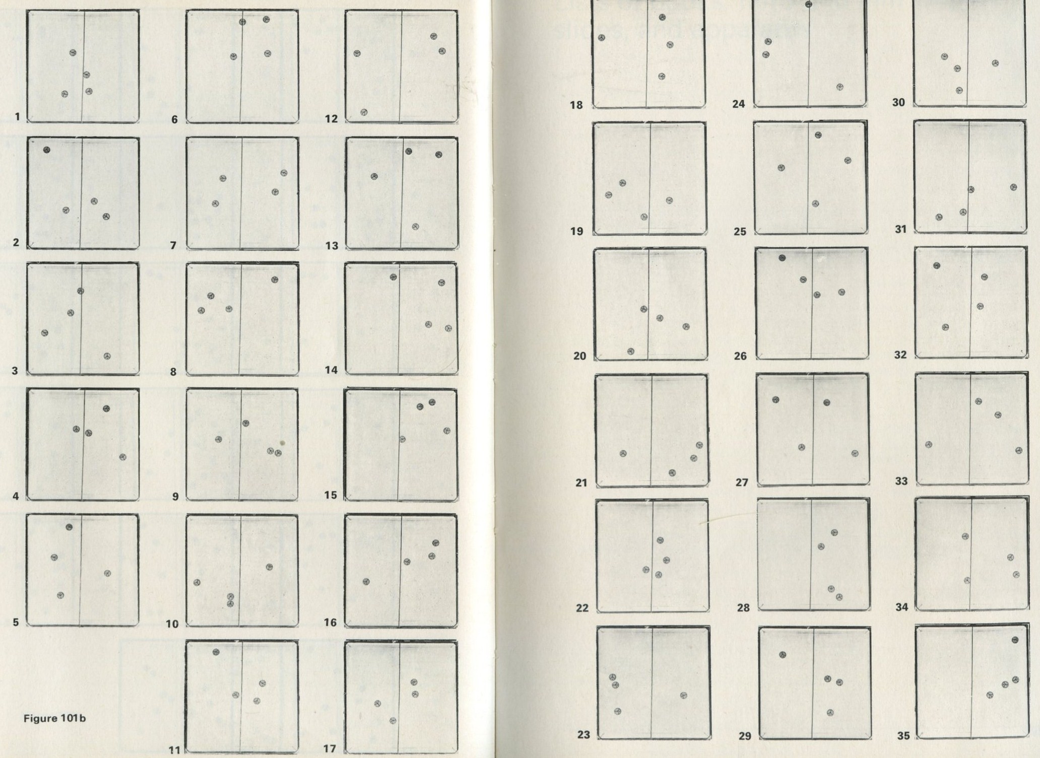
Figure 101b
List of books, films and film loops, slides and apparatus
Books
Page numbers of references in this book are emphasised.
Books for students
Angrist, S. W., and Hepler, L. G. (1967) Order and chaos. Basic Books. 23, 26, 28. This is a valuable book but it may be thought too expensive for the use it will have in this Unit.
Carnot, S. (reprint 1960) Reflections on the motive power of fire. Dover. 155. This is a translated edition, first published in 1890 with additional papers by Clausius and Clapeyron, of Carnot's original work of 1824 entitled Refexions sur la puissance motrice du feu.
Ogborn, J. (1972) Nuffield Physics Special Molecules and motion. Penguin/Longman. 99.
PSSC (1968) College physics. Raytheon. 99.
PSSC (1965) Physics. 2nd edition. Heath. 99.
Rogers, E. M. (1960) Physics for the inquiring mind. Oxford University Press. 99.
Sandfort, J. F. (1964) Science Study Series No. 22. Heat engines. Heinemann. 155.
Ubbelohde, A. R. (1954) Man and energy. Penguin. 23, 26.
Books for teachers
Bent, H. A. (1965) The Second Law. Oxford University Press. A book which we strongly recommend to any teacher using the Unit. 3, 15, 133, 188.
Campbell, J. A. (1965) Why do chemical reactions occur? Prentice-Hall. A simple, empirical, and clearly explained account of chemical equilibrium. 140.
Gurney, R. W. (1949) Introduction to statistical mechanics. McGraw-Hill. The first two chapters contain one of the first, and one of the best, simple introductions to statistical mechanics. 188.
Millen, D. J. (ed.) (1969) Chemical energetics and the curriculum. Collins. Useful for the links it makes with chemistry teaching. 188.
PSSC (1968) College physics. Raytheon. This book (but not PSSC Physics) contains the very interesting PSSC treatment of thermodynamic ideas. 132.
Reif, F. (1967) The Berkeley Physics Course, Volume 5 Statistical physics. McGraw-Hill. A useful book for those who want access to the ideas of statistical mechanics worked out thoroughly and in detail. It is pretty tough going in places. 188.
Sherwin, C. W. (1961) Basic concepts of physics. Holt, Rinehart & Winston. This book, regrettably out of print, contains a good, clear, and simple introduction to the ideas of statistical mechanics which teachers would find helpful. 188.
Sources of physics teaching Part 1 (1966) Taylor & Francis. Contains articles from Contemporary physics. This volume includes two articles on the introduction of the Boltzmann distribution. 188.
Nuffield Advanced Chemistry (1970) Teachers' guide II. Penguin. 141.
Films and film loops
16 mm films
Change and chance: a model of thermal equilibrium in a solid. 13½ minutes, black and white, silent. Penguin, XX1673. (Also available from Guild Sound and Vision Ltd.)
This computer-made film plays an essential part in the teaching of the Unit. It contains six short films on one reel, offered in this form rather than as 8 mm loops, for cheapness and clarity.
Random events 31 minutes, black and white, sound. Guild Sound and Vision Ltd, formerly Sound Services, 900 4116-5.
This PSSC film is not essential, but could prove a useful extra resource for the teaching of Part Three.
8 mm loops
'Forwards or backwards?' 1 Penguin, XX1668.
'Forwards or backwards?' 2 Penguin, XX1669.
'Forwards or backwards?' 3 Penguin, XX1670.
These three loops (in standard 8 only), produced for Nuffield Advanced Physics, play an important role in Part One of the Unit, though they could be replaced by other suitable film shown backwards.
Slides
The following is a list of slides for use with this Unit. They can be obtained from Penguin Books as a film strip under the title 'Unit 9 Change and chance', quoting the number XX1676.
9.1 World energy production and consumption
9.2 World fuel reserves
9.3 Total world rate of energy consumption
9.4 Cumulative world energy consumption
9.5 Total United Kingdom installed electrical generating power
9.6 Energy production. Africa
9.7 Energy production. North America
9.8 Growth of world population
9.9 Growth of number of cars in Britain
9.10 Energy account for cars
9.11 Power station with cooling towers (High Marnham)
9.12 Power station alongside a river (Belvedere)
9.13 The iodine molecular absorption spectrum
List of Apparatus
    2B   copper wire, 32 s.w.g. bare               9.6, 9.10, 9.14
     9   Malvern energy conversion kit             9.1
    12   two-dimensional kinetic model kit         9.2
    27   transformer                               9.7
    42   lever arm balance                         9.9, 9.10
  44/1   G-clamp, large                            9.10
  44/2   G-clamp, small                            9.1
   52K   crocodile clip                            9.13, 9.15
    59   l.t. variable voltage supply              9.9, 9.10
    67   Bourdon gauge                             9.11
    70   demonstration meter                       9.10
  71/2   dial for demo  meter, dc. dial 5 A        9.10
 71/10   dial for demo  meter, dc. dial 15 V       9.10
    75   immersion heater                          9.9, 9.10, 9.11
    77   aluminium block                           9.6, 9.10, 9.14
   94A   lamp, holder, and stand                   9.7
  132N   thermistor (R S Components Ltd TH3)       9.13
   133   camera                                    9.2
   171   photographic accessories kit              9.2
   176   1 2 volt battery                          9.1, 9.6, 9.9, 9.11,  9.14
   179   d.c. voltmeter (0-1 5 V)                  9.11
 191/2   fine grating                              9.7
 503-6   retort stand base, rod, boss, and clamp   9.7, 9.11, 9.13
   507   stop watch or stop clock                  9.11, 9.12
   508   Bunsen burner                             9.11, 9.13
   510   gauze                                     9.11, 9.13
   511   tripod                                    9.11, 9.13
 512/1   beaker, 250 cm3
                  9.12, 9.13, 9.15
   517   volumetric flask, 1 dm3 (1 litre)         9.12
   522   Hoffmann clip                             9.11
   533   bucket                                    9.12
   542   thermometer ( - 10 to 110°C)              9.6, 9.9, 9.11, 9.12, 9.13, 9.15
   543   chinagraph pencil                         9.11
   548   round-bottomed flask                      9.11
  1001   galvanometer (internal light beam)        9.6, 9.10, 9.14, 9.15
1003/1   milliammeter (1 mA)                       9.15
1003/2   milliammeter (10 mA)                      9.13
1003/3   milliammeter (100 mA)                     9.13
1003/5   ammeter (10 A)                            9.9, 9.11
1004/1   voltmeter (1 V)                           9.6
1004/2   voltmeter (10 V)                          9.11
1004/3   voltmeter (100 V)                         9.9
  1005   multi-range meter (25 V range)            9.9
  1023   solar motor                               9.6, 9.14
  1033   cell holder with U2 cells                 9.1, 9.13, 9.15
  1041   potentiometer holder                      9.15
  1051   Small electrical items
         preset potentiometer, 5 kΩ                9.15
         germanium transistor (e.g. OC 71)         9.13
  1053   Local purchase items
         card                                      9.6
         counter                                   9.3, 9.4, 9.5, 9.8
         cork piece (30 mm diameter, 10 mm thick)  9.13
         Polyfilla                                 9.15
         Sellotape                                 9.10, 9.11
         slab of expanded polystyrene              9.6, 9.10, 9.11
         Vaseline                                  9.13
    1054 Expendable items
         constantan wire, 32 s.w.g., covered       9.6, 9.10, 9.14
         copper wire, 14 s.w.g., bare              9.15
         film, monobath combined developer-fixer   9.2
         glass tube, 1 0 mm bore, 50 mm long       9.15
         graph paper                               9.3, 9.4, 9.8
         piece of porous pot                       9.11
         rubber pressure tubing                    9.11
   1055  Small laboratory items
         bung with 2 holes (thermometer,  T-piece) 9.11
         burette                                   9.11
         dice                                      9.3, 9.4, 9.5, 9.8
         flat-bottomed flask, 1 dm3 (1 litre)      9.12
         measuring cylinder, 100 cm3
                  9.10, 9.12
         specimen tube                             9.15
         teat pipette                              9.15
         test-tube, hard glass(150x25mm), with cork9.7, 9.11, 9.15
         T-piece                                   9.11
   1056  Chemicals
         1 M copper sulphate solution              9.15
         dextrose (glucose)                        9.12
         ethanol (ethyl alcochol)                  9.12
         formaldehyde                              9.12
         0.1 M hydrogen peroxide solution          9.12*
         iodine crystals                           9.7
         methylene blue                            9.12
         phenolphthalein                           9.12
         0.1 M potassium iodide solution           9.12*
         saturated potassium nitrate solution      9.15
         0.1 M silver nitrate solution             9.15
         silver wire                               9.15
         sodium hydroxide                          9.12
         sodium metabisulphite                     9.12
         sodium sulphite (anhydrous)               9.12
         0.01 M sodium thiosulphate solution       9.12*
         0.5 M sulphuric acid                      9.1, 9.12*
         0.2 % starch solution                     9.12*
         zinc dust                                 9.15
    1064 low voltage smoothing unit                9.9, 9.10
    1070 gas energy transfer apparatus             9.10
    1072 semiconductor thermopile unit             9.14

* Alternative version.
Index
Back Cover