Unit 9: Part 4

Contents

• 4. Thermal equilibrium, temperature, and chance
  • Thermal equilibrium
  • The zeroth law
  • An analogy: getting on with someone
  • Scales of temperature
  • The large scale and the small scale
  • A game of chess with quanta for chessmen
  • What happens in the game?
  • The distribution of quanta among atoms
  • The quantum shuffling game played with large numbers of atoms by a computer
  • Still pictures from the computer films of randomly shuffled quanta
  • What can be learned about thermal equilibrium from the computer films?
  • Summary: chance and the flow of heat
  • The absolute Kelvin temperature scale
  • The heat capacity of an Einstein solid
  • Constant thermal capacity for many elements
  • Dulong, Petit, Einstein, and heat capacities
  • Value of the Boltzmann constant k and mean energy per atom
  • The Boltzmann factor
  • Summary of Part Four
  • A place to stop

4. Thermal equilibrium, temperature, and chance

An improvement in our knowledge of heat, which has been attained by the use of thermometers, is the more distinct notion we have now than formerly of the distribution of heat among different bodies. Even without the help of thermometers, we can perceive a tendency of heat to diffuse itself from any hotter body to the cooler ones around it, until the heat is distributed among them in such a manner that none of them is disposed to take any more from the rest. The heat is thus brought into a state of equilibrium.

This equilibrium is somewhat curious. [Our emphasis.] We find that, when all mutual action is ended, a thermometer applied to any one of the bodies undergoes the same degree of expansion. Therefore the temperature of them all is the same. No previous acquaintance with the peculiar relation of each body to heat could have assured us of this, and we owe the discovery entirely to the thermometer. We must therefore adopt, as one of the most general laws of heat, the principle that all bodies communicating freely with one another, and exposed to no inequality of external action, acquire the same temperature, as indicated by a thermometer. All acquire the temperature of the surrounding medium.

By the use of thermometers we have learned that, if we take a thousand, or more, different kinds of matter - such as metals, stones, salts, woods, cork, feathers, wool, water, and a variety of other fluids - although they be all at first of different temperatures, and if we put them together in a room without a fire, and into which the sun does not shine, the heat will be communicated from the hotter of these bodies to the colder, during some hours perhaps, or the course of a day, at the end of which time, if we apply a thermometer to them all in succession, it will give precisely the same reading. The heat, therefore, distributes itself upon this occasion until none of these bodies has a greater demand or attraction for heat than every other of them has; in consequence, when we apply a thermometer to them all in succession, after the first to which it is applied has reduced the instrument to its own temperature, none of the rest is disposed to increase or diminish the quantity of heat which that first one left in it. This is what has been commonly called an equal heat, or the equality of heat among different bodies; I call it the equilibrium of heat.

From Joseph Black (1803), Lectures on the elements of chemistry. Reprinted in Conant, J. B. (1957) Harvard case histories in experimental science, Volume 1, Harvard University Press

Perhaps Joseph Black's discovery seems obvious or not very important. But it is important, because it is the reason why we can talk at all about the temperature of an object. First of all, in this Part, we discuss thermal equilibrium and temperature, as they appear to us on the large scale, and mention some of their practical implications. Then we shall try to get some idea of what thermal equilibrium is like, and what temperature means, when they are related to matter on the atomic scale, and to the energy shared amongst atoms.

Demonstration 9.6 A heat engine

The device shown in figure 21, a sandwich of semiconductor materials with cans on either side, produces enough electrical energy to turn a small motor if boiling water is poured into one can.

Figure 21: A thermoelectric heat engine.

More of something good may be better

But if cold water is put in the other can, the motor runs well, and, if ice is used, it runs even better. Indeed it will run if the hot can is filled with cool water from the tap as long as the other can is filled with solid carbon dioxide (dry ice). It will not run if each side of the device is equally hot or cool.

Q1 If the motor is running now, will it still be running in an hour's time? Why not?

Q2 Where does the energy to run the motor come from?

Q3 Why is there a heat flow from the hot can into the semiconductor sandwich?

Q4 Why is the sandwich cooler than the hot can?

Q5 Would the motor go on running if the cold can were not there?

Q6 Why must some heat flow into the cold can? Is this energy available to run the motor?

Q7 Is all the energy going out of the hot can into the semiconductor available to run the motor?

This engine cannot help but be inefficient to some extent. We shall return to the inefficiency of such engines later on, in Part Six, and outline why steam engines, petrol engines, gas turbines, and rocket engines must inevitably all be inefficient. We note now that temperature differences are useful, for they can be used to drive engines.

In this Part, we shall not pursue these points much further, but will use the engine to illustrate Joseph Black's discoveries about thermal equilibrium.

     1072     semiconductor thermopile unit 
     1023     solar motor 
     1004/1   voltmeter (1 V) 
      542     thermometers ( -10 to 110°C) 2 
      507     stop watch or stop clock 
      176     12 volt battery (to give 2V d.c.) 
     1001     galvanometer (internal light beam) 
     1054/2B  copper wire, 32 s.w.g., and constantan wire 32 s.w.g. 
       77     aluminium block 
     1053     slab of expanded polystyrene, Sellotape, card 
              supply of ice and of boiling water, salt, or solid C02 
     1000     leads 

Thermal equilibrium

Q8 Now imagine a film of the thermocouple device running a motor, but shown backwards. What would it seem to show? Say what energy transfers would seem to be taking place.

Interestingly, the reverse of the heat engine experiment can happen. The motor, run backwards as a dynamo, does not actually deliver enough current to produce an observable effect, so we replace it by a battery. When this is done, with equally cool water in each can, one lot of water grows warmer, and the other lot grows cooler.

This result may seem surprising, for we are all very accustomed to the inexorable one-way cooling down of hot things and warming up of cold things.

But if the battery is taken away, there are no surprises. Heat flows once again from the hot can to the cold can. A thermocouple connected to a meter, and placed alternately in each can, gives meter indications that are, at first, large but in opposite directions for the two cans. As time goes by, the two indications both become more and more nearly the same. See figure 23. Incidentally, the device is itself a thermocouple, but one between two sorts of semiconductor.

Note that so far as the conservation of energy is concerned (the basis of the First Law of Thermodynamics), energy could flow from cold to hot, as long as the same amount of energy left the cold object as reached the hot one.

Figure 23: Changes in temperature when the heat engine is reversed.

But, without external assistance, it never does. The approach to thermal equilibrium is one-way only. This is the theme of the Second Law of Thermodynamics, which will concern us more and more in this Unit.

Just now, we use the device to illustrate a third point, called the zeroth law of thermodynamics.

The zeroth law

What is thermal equilibrium? Objects in contact, like the warm and the cold cans, usually change their behaviour for a while. But soon all such changes stop, and the two are in equilibrium.

Suppose a third thing, such as a thermocouple, is put in contact with one can, and gives a certain reading. If it is put in the other, before the cans are in equilibrium, its reading changes. The couple was not in equilibrium with the second can. If it is put in the second can when the cans are in equilibrium, its reading doesn't change. The couple was already in equilibrium with the second can, just by being in equilibrium with the first.

Is this a long way of saying something very easy? Perhaps it is. But unless these things are so, measuring temperature is not even possible, indeed temperature means nothing. Suppose you used a thermometer whose indication is, say, 20°C, to find all those objects in a room which are at 20°C. That is, the thermometer indication stays put when it is placed in contact with them. Then the law we are thinking about says that none of them will change if they are put in contact with one another.

A set of objects of which we wish to say, all these are at the same temperature, must have something in common. And that something is that if they are put in contact, they will all be found already to be in thermal equilibrium.

This is called the 0th, or zeroth, law of thermodynamics. It is simple, but basic. If it were not so, a thermometer could give different readings for two things which were in equilibrium. Or perhaps one would find that of two things with the same reading, one of them was the hotter, because heat flowed from it to the other. Either event would make temperature measurement as we know it a useless procedure, because it would tell us nothing about the future behaviour of the bodies involved.

An analogy: getting on with someone

If A gets on well with B, and B gets on well with C, does A get on well with C? We could not be sure, so it would be impractical to think of measuring people so as to put each onto a scale of getting on well with others, and using the scale to predict who would get on with whom.

Q9 What does it mean, to say that two things are at the same temperature?

Q10 If two things are at the same temperature, do they contain equal amounts of energy?

Scales of temperature

Temperature exists is the message of the zeroth law. Making a scale of temperature, that is, putting a number to it, is a different matter.

Many scales have been invented, and many substances have been used in thermometers. Each scale, be it Celsius, Fahrenheit, Reaumur, or Kelvin, depends on deciding what number to assign to the temperatures of some things, such as ice, boiling water, or the lowest temperature possible, absolute zero. Each substance marks off by its changes, whether of volume, pressure, resistance, or some other property, the temperature between these fixed points. Any one thermometer can now be used to tell whether one object is hotter than another, according to how the physical property used to indicate temperature differs when the thermometer is put in contact with each in turn.

There remains, though, the question of assigning values of the temperature to the values of the physical property being used. If mercury in a thermometer placed in warm water can be seen to have completed half its expansion from ice temperature (0°C) to steam temperature (100°C}, it may seem sensible to assign the temperature 50°C on the mercury scale to that amount of expansion. But doing so is a matter of arbitrary decision, convenient but not absolutely necessary.

Furthermore. there is no guarantee that a coil of resistance wire, placed in the same warm water, will be found to have completed just half its increase of resistance from 0°C to 100°C. If the increase is less than half complete, the resistance coil temperature of the water will be (by the same decision) less than 50°C, disagreeing with the mercury expansion temperature.

These disagreements are usually not large, and their details are mainly important only in accurate work, or to thermometer designers. The existence of such disagreements indicates that we do not have here a fundamental basis for setting up a temperature scale. So we say no more about such temperature scales, though much of the rest of the Unit (especially Parts Four and Five) will pursue the problem of finding a fundamental basis for the idea of temperature measurement. This inquiry will lead us to the absolute, or Kelvin scale of temperature.

The large scale and the small scale

In the rest of this Part, we shall ask and begin to answer such questions as What is going on when things reach thermal equilibrium?, How do atoms come to share out energy so that the temperature is uniform?, and What is the difference between hot and cold so far as atoms in a body are concerned?

We shall be thinking about the large-scale (macroscopic) events discussed above and trying to form a small-scale (atomic, microscopic) picture of what is going on.

Einstein's model solid

To think about the questions raised above, we need to fix attention on something definite. It is no use trying to think about gases, solids, and liquids all at once, for each has its own rules for the motion and energy of its atoms. We need to find one definite picture of how atoms share energy in one kind of material. And it had better be as simple a picture as possible, to start with.

The best theoretical physicists often succeed because they can invent a really simple model which nevertheless gives useful ideas about complicated reality. It was Einstein who proposed the simple model we shall talk about. It is a model of a solid.

Q11 In a solid crystal such as sodium chloride, the ions are held in place by balanced forces acting on each ion. If one ion is displaced and released, how will it move?

Q12 Would you expect the oscillations of one ion to affect others nearby?

Q13 If all the ions in a row were oscillating in unison except one, what would you expect to happen to that one?

Einstein suggested thinking of atoms or ions as being fixed in place in a solid and vibrating as harmonic oscillators (remember Unit 4). In general they do not but it is much simpler to discuss their energy if we imagine a model in which they do. This is because such an oscillating atom can only have one of a series of definite energies, and these energy levels are equally spaced, like the rungs of a ladder. In Unit 2 you saw that there was experimental evidence that the electrons within atoms could be in only one out of a series of energy levels at a time. Those levels were not equally spaced. We are now talking about the energy of the atom when the whole atom is oscillating back and forth inside a crystal, not about the energy of electrons within the atom. These oscillation levels are equally spaced, if the oscillator is harmonic. The next experiment offers some experimental evidence to support this assertion. A theoretical reason to support the assertion can be found in Unit 10, Waves, particles, and atoms.

Einstein then introduced a further simplification that was very helpful, even though it was obviously wrong. It takes real cleverness to dare to do that, and to choose the right way to make the model wrong. The trick is to leave out those complications which won't affect the answers to the questions one is interested in (without knowing what those answers are!). Einstein's model achieves this for the answers we shall obtain.

Figure 24: Models of a solid

a A balls and springs model of a solid (later developed theoretically by Born and von Karman, in an improvement upon Einstein's arguments).

b Einstein's model, with nearly rigid prison cells around each oscillating atom.

Figure 24 illustrates this simplification. As the answer to question 13 suggests, the oscillations of one atom in a regular array, all linked by springy bonds as in figure 24 a, will affect the oscillations of others. In fact, figure 24 a is like a wave model of trolleys joined by springs (as used in Unit 4) but extended to two or to three dimensions. Indeed, those who developed Einstein's simpler arguments had to argue in terms of wave energy travelling all through the crystal. The trouble is that the energy levels of such linked oscillators affect each other so much that one cannot speak of the energy on one atom at all. Einstein's idea was to imagine the atom-oscillators not as if they were linked together but as if each were enclosed in a rigid prison cell, as in figure 24 b. But this was going too far, for then energy Would not be transferred from one atom to another at all, and there certainly would not be any heat flow to be discussed. So Einstein made the model a bit fuzzy at the edges, and allowed himself to imagine the walls of the prison cells as being just a little flexible, but not so much that the motion of one atom governed that of another nearby. Then energy could go from atom to atom, but the energy levels of each would be unaffected by the motions of any of the rest of the atoms.

Please don't think that Einstein proposed the model as a good way of imagining the arrangement of atoms in a solid. He proposed it as the simplest model he could think of which would still allow him to argue about heat flow and thermal equilibrium. As our present interest is in these matters, and not in the nature of solids, it is sensible to adopt the simplest possible model. But remember, although we shall talk of the energy of one atom, the model was invented to make that possible. For a real solid, it is usually not possible to think like that at all, and one must imagine compression waves travelling through all the solid and think of all the atoms sharing the energy cooperatively. (Real solids are like communist societies - all for one and one for all - while Einstein's model is like that simplified economic theory which supposes that there are many independent small manufacturers and shopkeepers, each acting independently of the rest, except for some flow of money between them. Their wealth can be counted up for each individual. In the ideal communist society the wealth belongs to everybody.) Some of the results of thinking about the model are true only for the model, but many are true of much more complex models, and just happen to emerge rather easily from the simple model. We shall try to make it clear which results are of each kind. Analogous arguments using models have appeared elsewhere in other Units.

Demonstration 9.7 A ladder of equal energy levels

We said that an atom vibrating like a harmonic oscillator has an energy limited to one of a series of equally spaced values. The energy level spacing is actually hf, where h is Planck's constant and f is the frequency the oscillator has in the ordinary theory of oscillators (2πf= √(k/m)) where k is the spring constant and m the mass).

Imagine the levels to be like the rungs of a ladder, as in figure 25. There is a lowest rung, rung zero, and others above it. If the atom passes from rung one to rung two it has to acquire one lump of energy, magnitude ε. But on another occasion it may pass from rung five to rung four: it then gives up the same amount of energy ε.

An oscillating atom may absorb the energy needed to jump from one level to another, from some light. hf (again) gives the energy absorbed, the frequency f being that of the light. A spectrum of light, that has passed through some oscillating atoms that have absorbed energy from it shows dark lines at particular frequencies f, and these frequencies yield evidence of the energies hf absorbed from the light. (In Unit 4 we argued about this for the absorption of infra-red radiation by sodium chloride.)

Figure 25: A ladder of levels

A solid, even a transparent solid, is quite unsuitable for showing the equally spaced ladder of levels. As we explained above, real solids are not much like the Einstein model made of many independent oscillators. For a demonstration of the ladder, the best thing to use is a gas of two-atom molecules, like iodine, I₂. Being in a gas, the molecules are nicely separated and don't affect each other's vibrations. Being made of two atoms, each molecule can vibrate in and out like two masses joined by a spring.

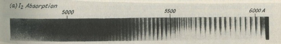
Figure 26: Part of the absorption spectrum of iodine vapour.

From Gaydon, A. G. (1968) Dissociation energies and spectra of diatomic molecules, Chapman & Hall.

Figure 27: Observing the iodine absorption spectrum.

Figure 26 is a photograph of the iodine vapour absorption spectrum. You can see the spectrum for yourself by looking at a filament lamp through a diffraction grating, and putting a tube full of iodine vapour in the way as in figure 27. The vapour is produced by warming the tube gently, there being one small iodine crystal in the bottom of the tube. The red, yellow, and part of the green regions of the spectrum are crossed by a ladder of many dark lines.

Figure 28 suggests how the ladder of lines arises.

Figure 28

In the warm iodine vapour, nearly all molecules are in the lowest state of electron energy, and many have the least possible vibration energy. A molecule can absorb energy by jumping to a higher state of electron energy, but the excited molecule can also vibrate in one of a ladder of vibrational energy levels. So there is a whole ladder of absorption lines corresponding to an electron jump, combined with a jump to one or other of the levels in the ladder of vibration energies that go with an excited state of the electrons in the 12 molecule. Ladders of levels give ladders of absorption lines.

      94A      lamp, holder, and stand 
       27      transformer 
    191/2      fine grating (about 300 lines per millimetre) 
     1055      test-tube, hard glass, 150 × 25 mm, with cork 
     1056      iodine crystals 
      508      Bunsen burner 

A game of chess with quanta for chessmen

The chess board (though it has only 36 squares) in figure 30 represents the array of atoms in a solid, each square, like each atom, having a fixed site within the whole.

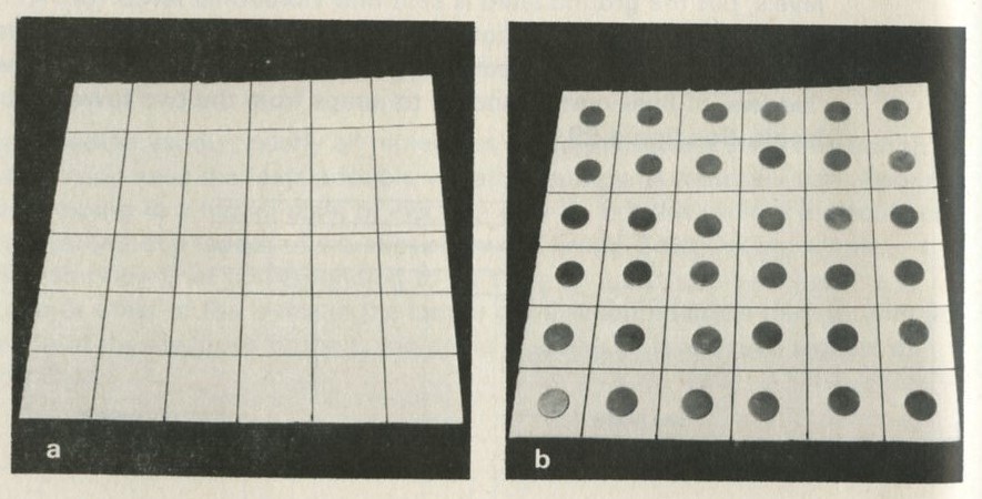
Figure 30: A chess board of atomic sites in a solid. Photographs Michael Plomer

Each square represents a site where there is an atom. The energy of an atom at one site will be represented by piling counters on that site. No counters on a site means that the atom at that site is in its lowest energy level. One counter is added to represent lifting it to the first level, another to represent lifting it to the next, and so on. Figure 30 a shows the 36-atom solid with each atom in its lowest level.

Figure 30 b shows it with each atom in the next level up, with one counter on each site.

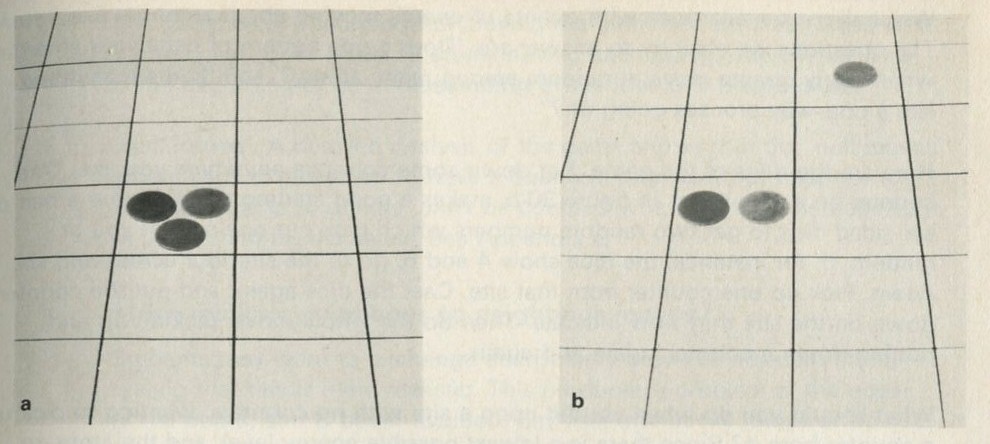
Figure 31: Transferring one quantum of energy. Photographs, Michael Plamer.

How shall we represent energy passing from atom to atom? The energy levels are equally spaced. Therefore, if a counter is picked up from an atom in the third level (with three counters, so that it then has two and has dropped one level), the same counter can be put down anywhere else and will represent the atom it now joins jumping up one level. Figures 31 a and b show one atom going from level 3 to level 2, and another going from the lowest level to the first level above that, all by moving one counter.

If a counter, representing one quantum of energy, were not put down once it had been picked up, the total energy would have decreased. It must go somewhere; to begin with we shall investigate what happens when the solid is well insulated so that no energy leaks in or out. So a counter picked up from one site must be put down on some site or other.

The fact that the counters representing quanta (which are real bits of plastic or metal) are distinct from one another, is not true of quanta. But the moves could just as well be made by keeping a paper and pencil tally of the state of each atom, remembering to move one atom down an energy level for every other atom one moved up one level. The plastic counters just save one having to remember or write down the state of each atom.

Game: 9.8 Moving quanta at random

How shall we choose which atoms gain energy and which lose energy? The clue to Understanding diffusion in Part Three was that there were no rules other than those of chance: if atoms move about quite by chance, then diffusion will inexorably happen if there are many atoms involved. A predictable, one-way diffusion process emerges from total atomic chaos.

We shall try a similar idea with quanta of energy moving about amongst fixed atoms. The questions we shall try to answer are, Does a tidy pattern of behaviour emerge when many quanta move at random among many atoms? and Is there anything like a one-way process going on?

Here are the rules of the game. Put down some counters anywhere you like. One counter on each site, as in figure 30 b, makes a good starting point. Throw a pair of six-sided dice to get two random numbers which pick out one site for you at random. If, for instance, the dice show 4 and 6, go to the site four across and six down. Pick up one counter from that site. Cast the dice again, and put the counter down on the site they now indicate. Then do the whole move, picking up and putting down a counter, again and again.

What should you do when you hit upon a site with no counters, wanting to pick up a counter from it? Since there is a lowest possible energy level, and the atom on that site is already in this level, it can go no further down. You will have to try again for another site, perhaps several times, until you find one with a counter to pick up.

The game does have definite rules. They are meant to achieve chaos. There are no rules saying where a quantum (counter) must go from each particular place: it may go anywhere. In that sense, there are no rules, or if you prefer, only that of chance.

    1053 counter (tiddlywinks are suitable) 36 
    1055 dice 2 
    1054 graph paper 2 sheets 

What happens in the game?

When you play the game you may notice a number of things. As you ought to have expected, the nice tidy one-counter-per-site pattern soon vanishes. And it never returns: the game leads, one-way only, away from such tidy patterns.

After about a hundred moves it is interesting to ask whether another hundred moves will make any more change. In one sense, obviously the answer would be yes. If you go on and on, some, at least, of the atoms which now have, say, two counters will have some other number of counters. The counters keep on moving. Yet, in another sense, not much more change happens, however long you go on after the first long run of moves.

Q14 Suppose you made the following records after 100 and 200 moves:

A the locations of sites with, say, two counters. 
B the number of sites with, say, two counters. 

Which record would be about the same each time, do you think?

The distribution of quanta among atoms

To start with, you may have had 36 sites each with one counter. No sites had no counters, and no sites had two, or any larger number of counters.

After a while, some sites have no counters, fewer than 36 have one, some have two, and so on. A good way to follow such changes is to plot bar charts with columns whose heights represent the numbers of atoms having no quanta, one quantum, two quanta, and so on. This is called the distribution of the atoms among the possible energy levels.

Figure 32: Twelve sample games (36 sites, 36 quanta, 100 moves) played by computer. a Initial distribution. b Distributions after 100 moves.

Figure 32 a shows what the bar chart looks like if you start with one counter on each atom - a single column 36 units high. Figure 32 b shows what happened to the distribution after 100 moves in each of twelve different trials of the game. Figure 33 shows the average of these twelve games.

Figure 33: Total of 12 computer samples (36 sites, 36 quanta, 100 moves in each sample).

Q15 Look at figure 33, or at the average of the bar charts obtained in your class. Suggest a rule about whether the numbers of atoms with n quanta will be more than, fewer than, or the same as with n + 1 quanta.

Q16 Is the difference between the number of atoms having four quanta and the number having three quanta the same as the difference between the number of atoms having one quantum and the number having none?

Q17 Speculate: what might be true of the ratios between the numbers of atoms in adjacent columns of the chart, but for chance variations because of the small total numbers involved?

Q18 Just before question 15, we introduced the term distribution. Figure 33 shows a distribution. To which aspect of figure 33 does this term refer?

• a The number of atoms with no quanta.
• b The collection of numbers of atoms with no quanta, one quantum, two quanta, and so on.
• c The total number of atoms.
• d The average number of quanta per atom.

Q19 Suppose one of next year's students were just starting to play the game.

• a Could you predict in advance which atoms would give or receive quanta?
• b Could you predict in advance anything about how the game would go?

The quantum shuffling game played with large numbers of atoms by a computer

Questions 15 to 19 may have brought out some of the results of the game of randomly moving quanta in an Einstein model of a solid. But because chance is at work and the numbers involved are small, the results vary quite a lot. So you ought to be doubtful about whether what you have seen is to be expected or is an accident. Ought the distribution to slope downwards towards higher energy states of atoms? Does it have a definite shape or not? If it does, what is the shape?

Such questions can only be answered by a trial with larger numbers of atoms and quanta (or by a theoretical discussion). Chance is like that: only trials with large numbers give reliable answers. A poll of ten people is a bad guide to how the country will vote in an election, but a poll of a thousand can be more reliable.

Sometimes it is possible to calculate in advance what to expect. This is possible for the number of times zero will turn up at roulette, but not for the number of votes in an election. It is possible to make such a calculation for the quantum shuffling game, but it is not easy. Part Five indicates how it may be done, and the calculation is given in Appendix B. For many problems, calculations are too difficult or impossible, and they are often tackled by making many random trials to see what happens. The problem of the most likely length occupied by a polymer molecule that can coil and uncoil at random, has been tackled in this way, for instance. This way of going about a problem is called, for obvious reasons, the Monte Carlo method. The advent of computers which can rapidly make many random trials according to certain rules has greatly increased the popularity of Monte Carlo methods.

We arranged for a computer to play the game you have just tried, but with 900 sites and 900 counters. The computer simultaneously made a film of what was happening in its head, so that you can see how the quanta move about and what happens to the bar chart showing the distribution.

Still pictures from the computer films of randomly shuffled quanta

In all, the computer made six short films, the series being called Change and chance: a model of thermal equilibrium in a solid. Figures 34 to 65 are still frames from the films, for you to inspect at leisure. (The frames are not prints from the film negative, but were made at the same time as the film, using the same data. The computer printed the pictures directly onto sensitized paper as well as onto film.)

Equilibrium of randomly shuffled quanta (figures 34 to 42)

In this film, the first, 900 atoms share 900 quanta, starting with one quantum on each atom. After making two moves in slow motion, to show that the rule used is the same as the rule we suggested that you should use in the game (9.8), moves are made at high speed until 10,000 moves have been made. The distribution has changed to a downward-sloping shape. Then a further 10,000 moves are made, during which the distribution fluctuates a little, but does not change its overall shape. Finally, the average distribution for the last 10,000 moves is calculated and displayed.

Figure 34: 900 atoms each with one quantum.

Figure 35: One atom is chosen as the first step in moving a quanta.

Figure 36: The atom chosen in Figure 35 loses a quanta.

Figure 37: An atom is randomly chosen to receive the quantum removed in figure 36.

Figure 38: The quantum removed from an atom in figure 36 is given to another atom. One move is completed.

Figure 39: 100 moves like those in figures 36 to 38 have been completed. Much of the original pattern still persists but several atoms have no quanta or two quanta.

Figure 40: The system of 900 atoms and 900 quanta after 5000 moves.

Figure 41: The effect on figure 40 of 5000 more moves. The distribution has not changed essentially, though individual atoms have different number of quanta.

Figure 42: The average distribution over the last 10,000 moves out of 20,000. The numbers over each column are the numbers of atoms having each number of quanta. Each is nearly twice as big as the next.

Different initial arrangement of quanta (figures 43 to 47)

In the second film there are still 900 atoms and 900 quanta, as in the first film, but the quanta are differently arranged at the start, to see if the starting point has any influence on the distribution reached after many moves.