
STARLINK used both GKS and GKS-3D on the STARLINK Vax machines. The joint Rutherford/ICL GKS implementation was enhanced by a set of routines relevant to the STARLINK community.
SGS is a set of subroutines which facilitates graphics output via the GKS package. GKS, which is described in the ISO document GKS 6. 2 and in SUN/11, is a device independent graphics system designed to be the kernel of a wide variety of graphics systems. It does not itself set out to provide the most convenient set of interfaces for all applications.
SGS, while preserving GKS concepts and indeed allowing direct GKS calls to be interspersed with SGS calls, is optimised for convenience in simple cases. Many of its features are low level (for example: open, draw a line, draw a text string, close), but there are some routines of a slightly higher level (drawing arcs and formatted numbers etc). SGS does not itself provide routines for high level operations like drawing annotated axes or complete graphs; these are facilities that will in due course be provided, using SGS as a basic support package.
Many plotting programs will be written entirely with SGS calls. There may, however, be occasions when GKS routines are required in addition, either because the GKS facility is sufficiently convenient in itself and has not been repackaged) or because a specialised feature of GKS is needed. Therefore the manual uses GKS concepts to describe SGS and the reference section (in Appendix A) describes SGS routines in terms of their effect on GKS. This will allow programmers to mix GKS and SGS calls without trouble. The unadventurous user may safely ignore (and indeed discard) the appendices.
The current version of CKS - 6.2 - is superseded by an implementation of the revised standard - 7.2. There are a number of important differences and changes will be needed to many GKS-based programs when the new implementation arrives. However, the revised GKS implementation that will be available at the same time will not, in general, appear to the programmer to have changed and so use of SGS now will obviate changes when the switch to GKS 7.2 is made. SGS has been designed with an eye on both these revisions, which is why one or two of the current routines contain very little code and why under 7.2 certain other routines will undergo considerable simplification.
The structure of this manual is:
This is a developing system and users are invited to make comments to any of the authors.
Programs that are to perform graphics I/O via GKS must begin by calling a sequence of GKS routines, and must call a similar number to close down the system. These calls have been conveniently packaged in SGS:
      CALL SGS_OPEN(WKSTN, IZONID, ISTAT)
      ...
      CALL SGS_CLOSE
The call to SGS_OPEN is mandatory for any program that will subsequently use any of the SGS routines, and all such programs should call SGS_CLOSE when plotting is complete. The arguments of the OPEN call are as follows. WKSTN is a the workstation name, a character string specifying the required graphics workstation. IZONID receives from SGS the zone identifier, a number allocated by SGS which we may need later to refer back to this workstation. ISTAT is the status, which will be zero if the OPEN has succeeded.
Friendly workstation names (e.g. 'PLOTTER') can be given to GKS workstations, either by the user or by the VAX system manager, and then specified in the SGS_OPEN call. The mechanism which involves VAX logical names, is described in SGP/26; consult the manager of your VAX about local conventions. Alternatively, the two numbers which GKS needs - the workstation type (what sort of device) and the connection identifier (which one) - can be given directly, as a character string consisting of 2 numbers separated by a comma.
The workstation type is currently one of the following:
  1    Sigma ARGS
  2    Tektronix 4O1O
  3    Sigma T5671
  4    Tektronix 4O14
  5    Versatec
  6    HP 7221 plotter
  7    Printronix
  8    Sigma T5674
  9    Calcomp 81 plotter
 10    Site dependent
 11    Cifer 2634
 12    HP 2648A
 15    Sigma ARGS overlay planes
100    Metafile output
200    Metafile input
300    Segment storage
(SGS merely passes this number to GKS, so any workstation type acceptable to CKS will do - refer to the current SUN/11.)
Broadly speaking, the connection identifier specifies which of several workstations of the nominated type is to be opened. For all but the Versatec and Printronix, use 0. For those cases, the connection identifier is the Fortran unit to which the output will be sent for temporary storage on disc, prior to output to the graphics printing services. The commands to send the file to the Versatek and Printronix graphics queues are:
      PRINT/QUEUE=GAAO filename           [Versatek]
      PRINT/QUEUE=GABO filename         [Printronix]
As an example, we are working on a Tektronix 4010 terminal. The required call is:
CALL SGS_OPEN('2,0', ITEK, ISTAT)
If, instead/ we wish to create a disc file suitable for plotting on the Versatec, we could use:
CALL SGS_OPEN('5,9', IVERSA, ISTAT)
If the default assignment for Fortran unit 9 is used, then after the program has completed, a print command can be issued to send the graphics data to the Versatec:
PRINT/QUEUE=GAAO FOR009.DAT
The purpose of the zone identifier will become clearer later on, suffice it to say at this stage that this number (which is allocated by SGS and cannot be set or otherwise processed by the user's program) allows the program to refer back to the full display surface of the workstation that has been opened.
Should any error messages be output by the SGS or GKS routines, they will be sent to Fortran unit 22.
It is a central philosophy of SGS that only one workstation should be active at once. However, multiple workstations may be open at once, and plotting may switch between them.
Successive workstations may be opened with calls to the SGS routine OPNWK:
CALL SGS_OPNWK(WKSm IZONID, ISTAT)
On each occasion that SGS_OPNWK is called, previously active workstations are deactivated before plotting switches to the new workstation. Thus, if the program is to plot first on a VDU then later on a plotter, it is best to open the plotter in the SGS_OPEN call and then to use SGS_OPNWK to open the VDU. Plotting on the latter can then begin.
Switching between multiple workstations is accomplished by the select zone routine which will be described in the next chapter.
If we want more flexible control - for example the ability to have several workstations active at once - this is available directly through the GKS activate/deactivate routines:
      CALL GKS_ACWK(IWKID)
      ...
      CALL GKS_DAWK(IWKID)
The GKS routine CLWK is available should selective close down of multiple workstations be required:
CALL GKS_CLWK(IWKID)
A final call to SGS_CLOSE will always leave the system correctly terminated.
(N. B. Direct calling of GKS routines will reduce the usefulness of the ID returned bu. SGS_ICURW.)
It is sometimes necessary to distinguish between different parts of a graph. There are a variety of ways this might be achieved, depending on the characteristics of the particular graphics device concerned: for example by plotting in different colours, or by using dotted lines, or by varying the line width. Individual control over all of these options is possible within GKS; the SGS package offers instead a simplified facility where one of a small number of clearly distinguishable line qualities may be selected, each specified by an SGS pen number. The call is:
CALL SGS_SPEN(NPEN)
where NPEN is the number of the SGS pen - an integer greater than or equal to 1.
SGS pen number 1 is the default, and is the normal pen for the device - a solid white line on a vdu, for example, or a black line of ordinary width on a plotter. SGS pens 1 to 4 may be assumed to be available and will correspond - depending on the device - to different colours or different styles of dashed line. Pen numbers greater than 4 may or may not be available depending on the device.
The last requested SGS pen number can be obtained by means of:
CALL SGS_IPEN(NPEN)
Detailed control over line colour, etc, is available via GKS and it is permissible to use these facilities. A call to SGS_FLUSH (about to be described) should precede any such activities. Note that revisions 6.2 and 7.2 of GKS differ significantly in these areas.
For efficiency, both SGS and GKS save up output in memory and send it to the graphics device in batches. Occasionally this may not be appropriate. For example an application program may plot a graph and then ask the user if the plot is satisfactory; it is clearly important that the whole plot must have been completed before user input is solicited. In such cases the call:
CALL SGS_FLUSH
causes any pending output to be sent immediately (to all active workstations).
An SGS zone is a block of display surface on a particular workstation, which behaves to some extent as if it were an independent plotting device.
A zone has an extent (in world coordinates), a position and size on the display surface (or, more correctly, in NDC) and a workstation. Clipping occurs at the zone boundary (unless disabled via GKS).
There are routines to create new zones and to switch plotting from the current one to another. When a zone is created it is allocated a zone identifier by SGS which is thereafter used by the program to refer to that zone. When a workstation is opened (in either SGS_OPEN or SGS_OPNWK), a base zone is created which occupies the whole display surface. This base zone has a world coordinate extent such that the square (0,0) to (1,1) fills it in at least one coordinate. A similar default coordinate system is set up whenever a zone is created.
One important use of the zone facility is to enable the allocation of plotting resources to be separated from the plotting itself. Thus the user might decide that the three graphs he is about to plot should, on one occasion, go to three regions of his VDU screen, and on another occasion to two regions of his screen and to a pen plotter respectively, by using zones the plotting program can operate as if the three plots were always on separate workstations, and switch freely between them during plotting. Activation and deactivation of workstations is handled automatically by SGS, as well as control of the various windows and viewports.
Another occasion on which SGS zones can be useful is when it is convenient to operate in several world coordinate systems within one graph. For example, a program might create one zone for plotting axes and annotation, and create one or more smaller zones within that zone for plotting data in world coordinates.
There is always a current zone, within which plotting occurs. Zones are created in terms of the current zone, with no restriction on the number of levels deep. Overlapping zones are permissible, but a new zone must lie entirely within the current one. There is a maximum number of zones that can exist at any one time, and a routine is available for dispensing with a zone once it is no longer required. There is no hierarchy of zones; once a zone has been created within the current zone and then made current, the parent zone can be released.
In all the create zone routines the new zone is selected, so that further plotting is to the new zone. The IZONID argument is the zone identifier supplied by SGS. ISTAT is the status return, which should be zero. The world coordinate system that the new zone is born with is such that (0,0) is at the bottom left hand corner, and (1,1) is on the top or right edge (or both). Thus the top right corner has one coordinate unity and the other unity or more.
A zone can be created within a nominated region of the current zone by means of:
CALL SGS_ZONE (X1, X2, Y1, Y2, IZONID, ISTAT)
X1, X2, Y1, Y2 are the bounds of the new zone, in the world coordinate system of the current zone.
A zone of nominated shape can be fitted into the current zone as follows:
CALL SGS_ZSHAP (AR, POS, IZQNID, ISTAT)
AR is the aspect ratio x/y. Thus a normal TV raster has an AR of about 1.3. The new zone has this aspect ratio, and fills the parent zone in at least one dimension. POS is a character string specifying the position of the new zone within the parent zone. The first character is 'B'* 'C' or 'T', to position the new zone at the bottom of the parent zone, centred vertically, or at the top. The second character is 'L', 'C' or 'R', for left, centre or right respectively.
For a zone of nominated absolute size:
CALL SGS_ZSIZE (XM, YM, POS, IZONID, ISTAT)
XM, YM are the dimensions of the new zone in metres. POS is as for SGS_ZSHAP.
Once a zone has been created (by SGS_OPEN. SGS_OPNWK or one of the above routines), it can be given a suitable coordinate system as follows:
CALL SGS_SW (X1,X2, Y1, Y2, ISTAT)
X1, X2, Y1, Y2 are the bounds of the current zone in the new world coordinate system.
To start plotting on a new zone:
CALL SGS_SELZ(IZONID, ISTAT)
Plotting is suspended on the current zone and the new zone, specified by the zone identifier IZONID, is made the current one. Subsequent plotting goes to the new zone. The selection may imply a change of workstation, this is handled by SGS.
There is only a limited amount of workspace within SGS for storing zone attributes, and it is best to release a zone once it is no longer required:
CALL SGS_RELZ (IZONID)
Attempts to release the current zone or the base zone for a workstation are simply ignored.
The zone identifier for the current zone is available via:
CALL SGS_ICURZ (IZONID)
To find out the size of the current zone:
CALL SGS_IZONE (X1, X2, Y1, Y2, XM, YM)
X1, X2, Y1, Y2 are the world coordinate bounds. XM, YM are the dimensions in metres.
To optimise plotting efficiency it is sometimes necessary for a program to find out what the plotting resolution is. The inquiry:
CALL SGS_IDUN (DXW, DYW)
returns the plotting resolution of the current zone, in world coordinates, in x and y separately.
The workstation identifier for the current zone may be required if GKS calls are to be employed. It is available by means of:
CALL SGS_ICURW (IWKID)
Many graphics packages have line drawing routines based on a current position concept. A single straight line is drawn either by calling first a set current position routine then calling a draw line from current position to new position routine, or by calling a general move routine twice with a pen up/down argument suitably set each time. The GKS line drawing primitive, on the other hand, does not use a current position but instead allows a series of connected straight lines, called a polyline, to be plotted as one item. The call is:
CALL GKS_POLYL(LENGTH, XARRAY, YARRAY)
where LENGTH is the size of the 1-dimensional arrays XARRAY and YARRAY, which contain the X and Y coordinates of the vertices of the polyline, in world coordinates. Thus the following code would plot a 3:4:5 triangle:
      ..
      REAL XA(4), YA(4)
      ..
      DATA XA/0.0,3.0,0.0,0.0/
      DATA YA/0.0,0.0,4.0,0.0/
      ..
      CALL GKS_POLYL(4, XA, YA)
      ..
However, there are times when this method may be inconvenient and an approach based on drawing single lines is more appropriate. In these cases, the SGS routines BPOLY, APOLY and OPOLY may be preferred. The BPOLY routine is used to begin a polyline:
CALL SGS_BPOLY(X,Y)
where X,Y are the starting coordinates for the polyline. The polyline is then built up by calls to APOLY, each of which appends a single line from the current end of the polyline to the new X,Y:
CALL SGS_APOLY(X,Y)
Finally/ when the polyline is complete, it can be output using:
CALL SGS_OPOLY
The triangle plotted in the example given earlier can be produced with the following code:
      CALL SGS_BPQLY(0.0, 0.0)
      CALL SGS_APOLY(3.0, 0.0)
      CALL SGS_APOLY(0.0, 4.0)
      CALL SGS_APOLY(0.0. 0.0)
      CALL SGS_OPOLY
In most cases the call to OPOLY may be omitted; any polyline awaiting output is automatically plotted if a new polyline is begun (via BPOLY or LINE) or at various other critical places within SGS.
It is, however, good practice to issue OPOLY if there is any uncertainty. For example, at the end of a general purpose subroutine is a good place, as the subroutine might be called in a case where keyboard interaction occurs before any subsequent line-drawing takes place. Redundant calls to OPOLY cause no problems.
      SUBROUTINE CROSS(X1, X2, Y1, Y2)
      REAL X1,X2,Y1,Y2
      CALL SGS_BPOLY(X1, Y1)
      CALL SGS_APOLY(X2, Y2)
*  CAN OMIT CALL TO OPOLY HERE  *
      CALL SGS_BPOLY(X1 Y2)
      CALL SGS_APOLY(X2, Y1)
      CALL SGS_OPOLY
      END
At any time, the current end coordinates of the polyline being built can be obtained by:
CALL SGS_IPLXY(X, Y)
(Only a limited amount of space is reserved for building the polyline; however, when this space is filled the polyline is automatically plotted and a new one begun starting from the last point given. Thus polylines of arbitrary length may be plotted via the SGS routines. Only if dotted lines are in use will the joins show. )
When the polyline to be drawn is merely a single line, it may be most convenient to use the SGS routine LINE, which opens a new polyline consisting of a single line:
CALL SGS_LINE(X1, Y1, X2, Y2)
The polyline begins at (X1, Y1) and ends at (X2, Y2). Note that output of the polyline is not forced, so the LINE routine can be used to begin a polyline of any length.
Rectangular boxes, with sides parallel to the axes, can be plotted by means of the SGS routine BOX:
CALL SGS_BOX(X1, X2, Y1, Y2)
The arguments are the x and y extents of the box.
The SGS package includes facilities for outputting both complete circles and arcs of circles:
      CALL SGS_CIRCL(X, Y, R)
      CALL SGS_ARC(X, Y, R,THETA1, THETA2)
The arc or circle is centred on X, Y and has radius R. The start and finish angles of the arc are THETA1 and THETA2 respectively, they are expressed in radians and have the conventional zero point and direction (e.g. an arc from 0 to PI/2 would begin at [X+R,Y] and end at [X, Y+R]).
There are a number of SGS routines for creating and plotting strings of characters. The most general, low level routines will be described first, although in many instances it will be more convenient to use the higher level routines TX, TXI and TXR, which allow single strings and formatted numbers to be plotted and which will be described later.
A text string can be plotted by means of the SGS routines BTEXT, ATEXT and OTEXT. BTEXT begins a new string:
CALL SGS_BTEXT(X,Y)
where X,Y is the position of the string (more about that shortly). ATEXT appends a new field onto the string:
CALL SGS_ATEXT(STRING)
and OTEXT outputs a completed string:
CALL SGS_OTEXT
The call to OTEXT can usually be omitted; any existing string is output automatically when BTEXT or CLOSE are called (and and at various other critical places within SGS).
(n.b. The maximum length of string that can be plotted is set by an internal workspace. Unreasonably long strings will suffer truncation to this maximum.)
There are several very useful higher level append routines.
The SGS routine ATXL appends a field to the text string after stripping any trailing blanks; thus if:
INITAL='S MCN '
the calls:
      CALL SGS_ATXL(INITAL)
and
      CALL SGS_ATEXT(INITAL(:5))
produce identical results.
The SGS routine ATXB, in contrast, appends a right justified field to the text string, but replaces any leading blanks with a specified number of blanks. Thus, if:
      NUM='      -0.035'
the calls
      CALL_SGS_ATXB(NUM,1)
and
      CALL SGS_ATEXT(NUM(4:))
produce identical results.
Routines are provided for conveniently plotting numbers; ATXI formats and appends an integer, and ATXR does the same for a real.
Integers may be plotted by. means of:
CALL SGS_ATXI(I,NFI)
where I is the number and NFI controls the formatting. If the number is to be left justified (for example within a message), an NFI value equal to the number of leading spaces should be specified. For example:
      CALL SGS_ATEXT('THERE WERE')
      CALL SGS_ATXI (25, 1 )
      CALL SGS_ATEXT(' SAMPLES')
would produce the string 'THERE WERE 25 SAMPLES'. If, on the other hand, right alignment is required (if a scale were to be marked on the left of a vertical axis, for example, an NFI value of minus the required field width should be specified.
Similarly, real numbers can be plotted with the SGS routine ATXR:
CALL SGS_ATXR(R, NFI, NDP)
where R is the number and NFI is as for the ATXI routine. NDP is the number of decimal places to be plotted. -1 (or any other negative value) causes only the integer part of the number to appear; if 0 is specified the decimal point appears as well; positive values result in the specified number of decimal places being plotted.
(n.b. Both ATXI and ATXR are limited in the width of fields they can handler and only sensible values should be used.)
Details of the text string under construction can be inquired through the SGS routine ITXB:
CALL SGS_ITXB (X. Y. N, DX, DY)
For the current zone, the ITXB routine returns the reference position (X,Y), the number of characters in the string (N) and the string extent (DX, DY). The string extent is such that if a new string is begun with reference position X+DX,Y+DY, it will append correctly to the current one, as long as the text attributes remain unchanged in between. The string extent works in this way if the default string alignment parameters are used (these are altered by SGS_STXJ - see below).
When the string to be output has already been formatted, or where a single number is to be plotted, it is convenient to use the SGS routines TX, TXI and TXR:
      CALL SGS_TX(X, Y, STRING)
      CALL SGS_TXI(X,Y, I, NFI)
      CALL SGS_TXR(X, Y, R, NFI, NDP)
In each case X,Y is the position of the string. STRING is the character string to be output, I and NFI are the integer to be formatted and the format indicator (exactly as for the ATXI routine); R, NFI and NDP are the real number to be formatted, the format indicator, and the number of decimal places (likewise exactly as for the ATXR routine).
These routines merely open a new text string and append the requested field to it; immediate output is not implied and more fields can be appended if desired.
The manner in which the text is plotted is controlled by a set of attributes, the most important of which are size, orientation and alignment. In addition, control over precision, font, aspect ratio and spacing is possible.
The size is specified by means of the SGS routine SHTX:
CALL SGS_SHTX(HT)
The argument HT is the height of the character box, in world coordinates (for upright text reading left to right). n.b. If the plotting scale (i.e. world units per mm) is altered, by calling SW for example, the character height will stay the same in world units and hence will change in mm. So if a given character height in mm is to be maintained across changes of the world coordinate system it will be necessary to call SHTX after each such change.
The orientation is specified by means of the SGS routine SUPTX:
CALL SGS_SUPTX(XU, YU)
where XU,YU is a vector specifying the up direction. The standard orientation is (0.0,1.0), for text on its side reading upwards an up vector of (-1.0,0.0) could be used, and so on. Only the vector, not its magnitude, is significant.
The disposition of the plotted string with respect to the reference x, y specified in the BTEXT call may be controlled using the SGS routine STXJ:
CALL SGS_STXJ(TXJ)
TXJ is a character string of length 2. The first character of TXJ is B, C, or T, and specifies whether the reference position is to lie on the bottom, centre, or top horizontal of the string. The second character is L, C, or R, and specified whether the reference position is to lie on the left, centre, or right vertical of the string. Thus a TXJ of BL (the default) will cause all strings to be plotted with the given X,Y at the bottom left corner. If CC is specified, all strings will be plotted centred on the given positions. (Notes: (1) The STXJ routine may be called at any time before the string is actually plotted and applies to all strings from then on. (2) The directions bottom, left, etc., refer to the string seen in its standard orientation.)
The SGS routine SPREC allows the text precision to be specified:
CALL SGS_SPREC(NPR)
A precision value of NPR=2 (the default) indicates that no avoidable discrepancy between the characters as defined by the font and as they appear on the display device is tolerable; in effect, software generated characters will be plotted which look the same on all devices. A precision value of 0 allows the use of hardware characters, a compromise between speed and appearance (the latter depending to some extent on how much trouble the user program goes to in order to find out the true extent of plotted strings).
Different fonts may be selected by means of the SGS routine SFONT:
CALL SGS_SFONT(NF)
where NF is the font number. The default font is ordinary letters and numbers.
Control of the aspect ratio of the character box is available via the SGS routine SARTX:
CALL SGS_SARTX(AR)
AR is the aspect ratio (width/height).
The SGS routine SSPTX allows the spacing between characters to be changed:
CALL SGS_SSPTX(SP)
SP is the distance between one character box and the next as a fraction of the width of the box.
The SGS routine IMTX allows all the above text attributes (as well as the marker height) to be inquired:
CALL SGS_IMTX(HM, NF, NPR, HT, AR, XU, YU, SP, TXJ)
A set of centred symbols, called markers, is supported. The symbol to be plotted is selected via a number called the marker type; the following set of markers is currently available:
type     symbol
 1         .
 2         +
 3         *
 4        square or O shape
 5         x
To plot a single marker, use:
CALL SGS_MARK(X, Y, MTYPE)
where X and Y are now single values.
Markers may be plotted at intervals along a polyline by means of the SgS routine MARKL:
CALL SGS_MARKL(MTYPE)
which plots the specified symbol at the current end of the polyline being built via APOLY. For example, the following code will plot a triangle with a star marker at corner A, an open symbol at corner B, and an X at corner C:
      CALL SGS_BPOLY(XA, YA)
      CALL SGS_MARKL(3)
      CALL SGS_APOLY(XB, YB)
      CALL SGS_MARKL(4)
      CALL SGS_APOLY(XC, YC)
      CALL SGS MARKL(5)
      CALL SGS_APOLY(XA, YA)
      CALL SGS_OPOLY
The marker height can be specified by the call:
CALL SGS_SHMK(HM)
where HM is the height (=width) of the symbol.
The current marker size HM (as well as all the text attributes) can be found via the SGS routine IMTX, which is described under text attributes.
SGS provides two ways in which a program can interact with the person running it; a graphics cursor (locator in GKS terminology) which the user can move around the screen with for example a joystick or trackerball and whose position in world coordinates can be read by the program, and a choice device in which the user selects one of a number of alternatives usually by pressing, a button on a control box or a key on a keyboard. The most familiar form of interaction is where the cursor is displayed and the program waits for the user to move it to the desired position and press one of the choice keys. The cursor position (a position in world coordinates) and the choice selected (a positive integer) are then returned to the program.
This type of interaction is achieved by:
CALL SGS_REQCU(X, Y, N)
If this routine is called repeatedly the cursor will reappear at the position that it was left at by the previous call. The cursor's position can be explicitly set by:
CALL SGS_SETCU(X, Y)
provided that the hardware allows the position of the cursor to be controlled by the computer. Not all devices have cursors, eg. the Versatec, and so a program can find out if the workstation of the current SGS zone has a cursor (all SGS input routines operate on the currently selected SGS zone) with:
CALL SGS_ICUAV(AVAIL)
where AVAIL is set to the logical value .TRUE, or .FALSE.. The cursor can also be used in a mode (sample mode) in which the cursor can be moved around by the user but the position is read by the program without waiting for the use to press a choice key. This mode of operation has to be explicitly enabled with:
CALL SGS_ENSCU
the cursor position can then be sampled with:
CALL SGS_SAMCU(X, Y)
typically in a loop. Sample mode is disabled with:
CALL SGS_DISCU
It is sometimes desirable to use this mode without the cursor being visible, its position being indicated in some other way such as continuously drawing a line to the cursor position from its position when last sampled. In order to allow this the cursor can be made invisible by:
CALL SGS_CUVIS(.FALSE.)
and made visible again with:
CALL SGS_CUVIS(.TRUE.)
The cursor will of course only actually appear if sample mode is enabled or when REGCU is called. Some hardware may not support the setting of the cursor visibility or the elegant operation of sample mode.
The choice device, which can be invoked either in conjunction with the cursor or on its own, can be one of two devices. By default it is a choice device associated with the graphics workstation such as the trackerball buttons on an ARGS or the numeric keys on a graphics terminal and is characterised by having a small number of choices (eg. only 4 on an ARGS). SGS provides an alternative device which is the keyboard of the terminal from which the program is being run. This has the advantage of being always available (except in a batch job!) and of having a much larger number of choices. However, since it is potentially a different device from the graphics device two separate read operations are required to get the choice and the cursor information and on a very busy system or over a network these operations may be separated by an appreciable length of time.
The choice device you wish to use is selected by:
CALL SGS_SELCH(NCHDEV)
where NCHDEV is 1 for the normal GKS device and 2 for the command terminal keyboard. The number of choices on a choice device can be inquired with:
CALL SGS_INCHO(NCHDEV, N)
If the choice device does not exist N will be returned as zero. The mapping of the keyboard keys onto the integers returned by SGS_REGCH is controlled by:
CALL SGS_DEFCH(CHOSTR)
where CHOSTR is a character string specifying which keys are to be considered to be valid choices. If the first character in the string is pressed an integer 1 will be returned, if the second a 2 will be returned, and so on. If the key is not included in the string a zero will be returned. There is no restriction on which characters can be specified but upper and lower case characters are not distinguished and you are advised to only use the FORTRAN character set (A-Z 0-9 =+*'.(),.:$ and blank) as other characters cannot be guaranteed to be present on a terminal. For this reason, if the number of choices on device 2 is inquired 49 is returned.
A typical use of this facility might be a program which plots a star field and then asks the user to identify each object on the plot as either a star a galaxy or a plate defect by positioning the cursor on each object in turn and pressing the S G or D keys to indicate the nature of the object or the "." key to terminate the sequence. The interactive part of this program might be
*    Select terminal keyboard as choice device
      CALL SGS_SELCH(2)
*   Define valid keys
      CALL SGS_DEFCH('SGD. ')
100   CALL REGCU(X, Y, N)
      GO TO (200,300,400,500) N
*  Not a valid choice (N is 0) try again
      GO TO 100
*   A Star
200   ...
      GO TO 100
*   A Galaxy
300
      GO TO 100
*   A Defect
400   ...
      GO TO 100
*  No more objects ..
500   CONTINUE
It is a Starlink recommendation that you use the "." character to terminate a sequence of operations such as this.
Your program can be linked using a logical name:
LINK objmodule.@SGSLINK
which loads both SGS and GKS, or the linking can quote the SGS library explicitly, in which case GKS must be quoted too:
LINK objmodule,LIBDIR: SGS/LIB,GKSOPT/OPT
There are no special requirements for running SGS other than those needed by GKS. The GKS workstation description table will be accessed automatically through the logical name GKSWDT. For full details see the latest version of SUN/11.
The routines are described in alphabetical order.
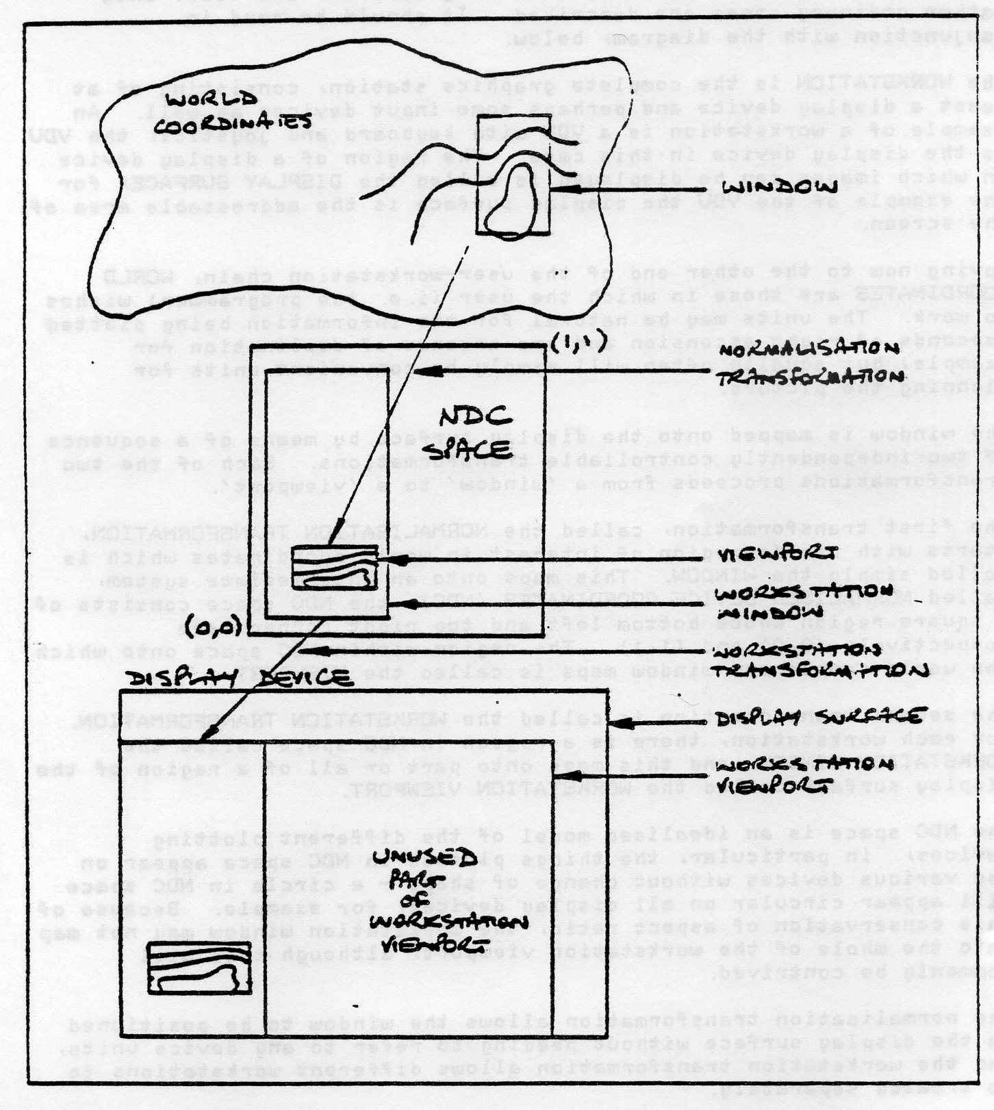
In the discussion that follows, (i) all the coordinate systems mentioned will be 2-D and rectangular, (il) official GKS terms mill be given in capitals when they are being defined, and (iii) only rather ordinary cases are described. It should be read in conjunction with the diagram below.
The WORKSTATION is the complete graphics station, consisting of at least a display device and perhaps some input devices as well. An example of a workstation is a VDU with keyboard and joystick; the VDU is the display device in this case. The region of a display device on which images can be displayed is called the DISPLAY SURFACE; for the example of the VDU the display surface is the addressable area of the screen.
Moving now to the other end of the user-workstation chain, WORLD COORDINATES are those in which the user (i. e. the programmer) wishes to work. The units may be natural for the information being plotted (seconds of right ascension and arc seconds of declination for example) but equally often will simply be convenient units for planning the picture.
The window is mapped onto the display surface by means of a sequence of two independently controllable transformations. Each of the two transformations proceeds from a 'window' to a 'viewport'.
The first transformation, called the NORMALISATION TRANSFORMATION, starts with user's region of interest in world coordinates which is called simply the WINDOW. This maps onto an intermediate system, called NORMALISED DEVICE COORDINATES (NDC); the NDC space consists of a square region whose bottom left and top right corners are respectively (0,0) and (1,1). The region within NDC space onto which the world coordinate window maps is called the VIEWPORT.
The second transformation is called the WORKSTATION TRANSFORMATION. For each workstation, there is a region in NDC space called the WORKSTATION WINDOW, and this maps onto part or all of a region of the display surface called the WORKSTATION VIEWPORT.
The NDC space is an idealised model of the different plotting devices; in particular, the things plotted in NDC space appear on the various devices without change of shape - a circle in NDC space will appear circular on all display devices, for example. Because of this conservation of aspect ratio, the workstation window may not map onto the whole of the workstation viewport, although this will commonly be contrived.
The normalisation transformation allows the window to be positioned on the display surface without needing to refer to any device units, and the workstation transformation allows different workstations to be treated separately.
At any time there can be only one window, NDC space and viewport, but there may be multiple display devices, each with its own workstation window and workstation viewport.
This appendix consists of a complete program using SGS. This and another (longer) program are available on disc in the files LIBDIR:SGSX1.FOR and SGSX2.FOR.
      PROGRAM SGSX1
*     --------------
*      S G S X 1
*     --------------
*   USES SGS PACKAGE TO DRAW BOX WITH 'STARLINK' WRITTEN IN IT
      CHARACTER*20 WKSTN
*  GET WORKSTATION TYPE AND NUMBER
      PRINT *, 'WORKSTATION?'
      READ (*, '(A)') WKSTN
*  OPEN
      CALL SGS_OPEN(WKSTN,IZONID, J)
*  DECLARE A SQUARE ZONE
      CALL SGS_ZSHAP(1.0,'O',IZ,J)
*  BOX
      CALL SGS_BOX(0.1, 0.9, 0.4, 0.6)
*  MESSAGE
      CALL SGS_SHTX(0.1)
      CALL SGS_STXJ('CC')
      CALL SGS_BTEXT(0.5, 0.5)
      CALL SGS_ATEXT (' STARLINK')
*  WRAP UP
      CALL SGS_CLOSE
END
