
This section of the book gives an informal description of the ATLAS computer system; both hardware and software are considered at the same time as the ATLAS system depended on both of these. The first few parts of this section provide an introduction to the operation of any computer system and various concepts, essential to the description of ATLAS, introduced. The later parts of this section give descriptions of the ATLAS system and include descriptions of the one-level store, the central processing unit (the mill) and of some of the peripherals on the machine.
How the user used ATLAS is described in a later chapter.
A description of some of the software that was generally available on ATLAS is also given.
Basically, all computers can be considered in terms of a simple model machine which has five basic units. Diagram 2 outlines the structure of such a model computer.
In the early days of computing, the typical machine could easily be completely classified in terms of this model (Pegasus, for example). Let us summarize the uses of each of the basic five units in turn.
The STORE UNIT holds all the information that is going to be used. Most usually, this information is held as a pattern of binary digits, the pattern being deduced for the information by some mapping function, arithmetic or otherwise. The store unit itself is divided up into individual store cells, each of which may hold a unit of information. Each store cell has associated with it an identifier, known as its address, and this is used to reference that store cell. Usually the non-negative integers are used for addresses with cells i and i + 1 being adjacent.
The MILL is the part of the machine where all the computations are carried out. Very often this unit has associated with it a set of store cells used to hold results and operands for the calculation: these are known as registers or as accumulators The mill will usually have the mechanism to carry operations such as addition, subtraction, multiplication, division, shifting, logical operations, loading and storing registers, testing etc.
The CONTROL UNIT is the most important part of all in any computer system. It is, in the same sense as the human brain, the nerve centre of the whole machine. Conceptually at least, this unit has inside it two special cells known as the program counter and the order register. The program counter holds the address of the store cell which contains the next order to be obeyed, while the order register holds the order currently being carried out.
Control is responsible for organising and initiating the execution of stored program by the machine and it does this by following a built-in procedure usually known as the execution cycle. On some modern micro-program controlled computers, this execution cycle is a micro-program in the micro-program control store. Basically, the execution cycle would operate as follows:-
In many machines the execution cycle is much more complex than this, but the added complications are only due to additional features that exist on such machines.
The INPUT DEVICE on early machines, and on this simple model, only transfers single characters from the input media to a store cell. The OUTPUT DEVICE is exactly similar, taking a single character from a store cell and putting this out.
As technology developed computers became faster and faster, and certain problems which were hidden by the slow speed of the earlier machines became more apparent. The most serious problem was the large amount of time lost in waiting for Input-Output operations to be performed. In a large data processing system, for example, it was found that the very expensive computer was spending a lot of its time waiting for input and output to be performed by comparatively slow peripheral units. Thus, if the machine was next to obey an order of the form
read a character from the paper tape reader
It would, following its execution cycle, load the order register with this order, increment the program counter, then obey the order in the order register. This would involve:-
sending a signal to the paper tape reader to get the next character, then waiting while the tape reader moved the tape along, read the next character, put it into the store and finally sent a message to control saying finished.
Control could then proceed with its execution cycle. A lengthy process! As the speed of the computer's electronics increased, it became more apparent that a lot of this time was being spent waiting for very slow mechanical devices to do their tasks. (very slow in fact should be regarded as comparative to the speed of the electronics of the computer).
Economically, running a highly expensive machine like this was disastrous as for much of the day the expensive electronic part of the machine was sitting idle.
Several methods were considered to try and solve this problem and reduce the amount of time spent waiting by the computer. It was observed that by using high speed peripherals such as magnetic tape units which could supply more information at a higher rate, that the amount of time spent waiting was dramatically reduced. It was this fact that inspired the famous IBM FORTRAN MONITOR SYSTEM. This system replaced all the slow peripherals, such as paper tape, punched cards, line printers on the main computer with the faster magnetic tape peripherals. A much smaller (and cheaper) computer was then installed and all the slow peripherals were connected to this machine, together with some magnetic tape decks. The information was then input from the slow peripherals to the small computer which output the information onto magnetic tape.
The magnetic tape was then transferred to the main computer which took all its input from this tape. A similar method was used for output, the main computer outputting to magnetic tape and the smaller machine being used to convert this to hard copy. The large machine then spent much less time waiting around for input, since magnetic tape was much faster than any slow peripheral and only a small, much cheaper, machine was used to drive the slow devices - far more economical.
The next improvement in the use of machine was due to the invention of the CHANNNEL. Even with magnetic tape being the input/output media, the main computer still had to wait while the transfer of data took place. The CHANNEL, however, allowed the peripheral device connected to transfer its data autonomously into the store leaving the main computer free to perform another task. The completion of the transfer was indicated by the CHANNEL setting a flag which the main computer could be programmed to interrogate. Thus a fragment of program for this sort of system could be:
          START I-O CHANNEL 1
          . . .
          . . .

Label 1.
         other processing
         . . .
         . . .
         IF CHANNEL 1 NOT FINISHED JUMP TO LABEL 1.
         . . .
         . . .
This allowed the main computer to carry out some task while the transfer was being undertaken. However, it did mean that programs had to be written in such a way that they asked for their input well in advance of using it and did not use the input until the transfer complete flag had been set by the channel. This placed quite a large responsibility on the programmer, making much of his work tedious.
The invention (or perhaps discovery is rather more accurate) of the INTERRUPT helped to make the use of channels easier. An interrupt is best thought of as a break in the execution of a routine in such a way that control is passed to some other routine (known as the Interrupt Service Routine) which can take the necessary action and then, perhaps, restore control to obeying the interrupted routine, so that it could continue execution as if nothing had happened. Thus when a CHANNEL had completed its transfer it would set its transfer complete flag but instead of waiting for this to be examined, the setting of this would cause an interrupt to occur. Control could then be transferred to a routine to deal with the end of the transfer, then return control to the point of interruption.
While this helps to make programming more simple it does mean that the programmer still must request his input well in advance, so that it will be input and present before he tries to use it. This means that he must either still examine a flag to check that his input is present or he must issue his read request and wait until the input of his data is complete. Now, the whole point of this sophistication was to obtain better utilisation of the main computer, so the idea of sharing the main computer between two (or more) programs developed.
In principle, the idea of multi-programming a single computer with several different programs is fairly simple: each program runs in turn until it is unable to do so any longer (i.e. waiting for input or some other event), so then another program is allowed to use the central machine until the input operation is completed, then the first program is allowed to continue again. Obviously, there must be some controlling program which arranges the swapping of programs: this program is usually known as the monitor program, executive program or operating system.
Monitor programs actually started their development as a set of useful routines to aid programming. With the advent of interrupts their role became far more important as there had to be some reliable controlling routine to ensure the smooth operation of programs. The early monitor routines provided easy input-output facilities, allowing the ordinary programmer to be unaware of the problems of waiting for input, and observing special flags. As computers evolved, so did operating systems - they began to deal with certain error conditions signalled to them by the hardware via an interrupt, for example, divide by zero errors, etc.
One of the most important of the early monitor systems was the Ferranti Orion Time-sharing System. From the sales description of ORION, we quote:
The time-sharing system ensures that:-
- the computer is always doing useful work
- peripheral devices are always kept working at their full speed
Every time that a peripheral transfer is finished, and every time the computer attempts to refer to data involved in an uncompleted transfer or to any equipment involved in such a transfer, then the time-sharing system processes the programme (sic) priorities in the store of the machine and decides whether to continue the operation of the present programme or to switch to another programme.
In general, the computer will switch to the programme of the first priority which is not waiting for the completion of a peripheral transfer.
When Orion reaches the end of a problem or a batch of data, it will not stop as previous computers would have done. In place of a stop order there is an intentional entry to the Monitor Routine. The Monitor Routine will carry out appropriate changes to the programme priority list, and continue with the remaining programmes or read in another.
The priority-processing is fully automatic, as are the arrangements for ensuring that programmes do not interfere with one another. The programmer does not have to concern himself with these matters when writing his programme.
By now it should be becoming clear that there are two main directions in which computers develop: along the lines of better hardware and along the lines of better software (programs). These two, are very much inter-related. We observe that The programmer does not have to concern himself..... There is now this helping hand between the real machine (the hardware) and the machine for which the user writes his programs, the helping hand being the operating system.
In describing any post-ORION computer one cannot really separate the hardware and its operating system, the two are for better or worse married together to provide the virtual computer that the user sees. How different this virtual machine is from the real machine (i.e. hardware alone) depends largely upon the System (i.e. hardware plus Operating System). We may consider the virtual machine in terms of the simple model set out earlier: every virtual machine will have its store, mill, input device, output device and control unit. Several virtual machines may exist and share the same real machine at the same time, but obviously there are problems involved in this sharing.
As we proceed to examine the ATLAS system we will do well to keep these early ideas in mind, observing the way in which both the hardware and software come together to provide the user's virtual machine.
Just as in the model computer described previously, on ATLAS the user saw a very large store built out of store cells, most of which he could use, but parts of which he could not use.
Most British computers before ATLAS only possessed a fairly small store unit which could hold between 55 (Pegasus) and 4096 (Orion) words of information. It was from this store that all the orders were obeyed and where all the datum values had to be held for a computation. For most purposes this store was far too small so an additional unit, known as the backing store was added to the system.
The backing store could really be considered as an input/output organ, its function in life being to provide supplementary storage space for data and program. In real computers this device is most frequently a magnetic drum or disc and information is transferred from the store onto the backing store and from the backing store into the main store.
The purpose of the backing store unit is to allow programs which will not fit into the main store alone to be run on the computer. The program has to be written in such a way as to need only part of its data or code, or parts of both, in the main store at any time. Programmed orders are explicitly written to transfer routines and data between the main store and backing store: these techniques are known as overlaying.
It should be remembered that orders are only obeyed, and data operated upon, from the main store and if anything held in the backing store is needed it must first be transferred to the main store.
Machines which had these two stores, a main store (or immediate access store) and a backing store, were said to possess a two-level store; the user saw two distinct types of storage, one was immediately accessible, the other having a latency time associated with it, and the user had to wait until information was transferred from this backing store to the immediate access store before he could use it.
ATLAS 1 provided the user with a one-level store, that is, the user programmed the machine as if all the store was immediate access store. This was (and still is) a great step forward. The programmer did not have to concern himself with the problems of deciding which part of his program need or could be overlayed since he has been provided with this large (in fact, huge for its time) store which he could use as he pleased.
There were certain parts of this one-level store that were forbidden from user access but we shall mention these later.
Each store cell in the one-level store accessible to the user consisted of forty-eight data bits and were arranged in groups of 512 cells, known as blocks. Addresses within the whole of the store (including those parts inaccessible to the user) consisted of twenty-four bits and had the format
The first 12 bits (0 - 11) held the block number and the nine bits (12-20) the word within this block field. Bits 21 - 23 were used to hold the character address (and were used only in certain orders). The top three bits of the block field (0-2) were used to say which part (either a legal to user part or illegal to user part) of the store was being accessed.
How was this huge store provided? In fact the ATLAS hardware was very special and together with some sophisticated software provided this one-level store using a technique known as paging. The ATLAS computer was the very first computer to have paging of any sort, and this was, in fact, one of the major advances made in the design of ATLAS over any other machine.
The ATLAS hardware consisted of a fairly large (for its day) immediate access magnetic core store (of 16 or 32K words) and a backing store of four 24K words magnetic drums. Each store cell consisted of 48 data bits and one parity checking bit, (thus the user saw the actual store cells directly). The immediate access store was divided into groups of 512 store cells, each group being known as a page. A store cell could be identified as cell iof page p, where 0 ≤ i ≤ 511 and 0 ≤ p ≤ 63 (for the 32K machine). It will be noticed that the word within block range of the virtual address is identical to the word within page range, and that the block range is much longer than the page range. On ATLAS 1, store cell addresses were 14 bit long, viz.
and virtual address (i.e. those produced by a program) were 24 bits long, viz.
Obviously, there must have been some method by which one was transformed to the other. We notice that here there is a transformation between the virtual processor (the one the user sees) and the real processor (the actual hardware).
When we are transforming something as basic to a computation as the addresses it uses, then this must be carried out at very high speed so that the virtual processor will run at an acceptable speed. It was to this end that ATLAS 1 was provided with very special hardware to achieve this address transformation.
We must also observe that the immediate access store was too small to accommodate all the blocks that the user may use - where were the blocks which would not go into the immediate access store kept? In fact, this is fairly simply answered, the blocks were stored either on one of the drums or in the main core store. We shall consider the accessing of a word in the one-level store, observing how the address transformation is achieved.
Suppose we consider a virtual address of the form:
The transformation operates as follows:-
The L field of the virtual address (bits 12 - 23) are passed directly through the transformation unit unchanged. The block field is transformed into the page number of the main store page where the block is presently residing.
A special inverse table of 64 (for the 32K machine) 12 bit words was held in the machine. There was an entry for each core store page of the machine, in this table, which held the block number which was currently residing on that page of the store. This table was looked up associatively, that is by contents, with the block number, to find which page on which the block being accessed currently resided. In normal table look-up, the key that is being looked up is used as the offset from the base of the table, but in associative look-up the key is compared with each of the entries in the table in turn until an identical entry is found, when the offset of this entry is then given as the looked- up value. (This look-up may take place in parallel and did on ATLAS.)
So then, the incoming virtual block number was looked up associatively and one of two events then occurred. Either there was non-equivalence, i.e. there was no entry in the table corresponding to the virtual block being looked-up, in which case a paging interrupt was signalled, or there was equivalence, i.e. the virtual block number had been matched with an entry, in which case the offset of that entry in the table was known and used as the page field of the real address. The top fifteen bits of the transformed address (0 - 14) were then used as the address for whatever operation was being carried out. The low 3 bits (15 -17) of the transformed address are never presented to the core store but are used in certain extra code routines.
We mentioned earlier that the real processor was shared amongst various virtual processors (i.e. several user programs were multi-programmed together) and also mentioned that all virtual addresses were 24 bits long, so to allow this sharing it had to be ensured that each virtual processor accessed only those parts of the store which had been allocated to it.
This could have been achieved by dividing the virtual store into partitions and allocating one partition to each user, but this would have meant that some sort of re-location of code and data would need to have been performed. A far better way was devised and used on ATLAS. This was to allow each virtual processor to have an entire virtual address space to itself. Thus, it was possible then for two distinct blocks belonging to two separate processes to have the same number. Mechanisms had to be provided on ATLAS to allow this sort of situation to be resolved successfully. In order to allow the above, what was really essential was that on block look-up in the associative table, the only blocks in the table that should be seen were blocks belonging to the program (i.e. virtual processor) that produce the address under consideration. On ATLAS there was, in fact, an additional bit for each entry of the associative table which was set to a 1 when that entry had to be ignored from the look-up process. These bits, known as the lock-out bits were controlled by the supervision routine that dealt with program swapping.
It should be pointed out that the associative table lookup was performed very quickly indeed by comparing the block field in parallel with the entries of the associative table. Diagram 4 shows the principle of the operation of the associative table mechanism.
Let us pursue the case where non-equivalence occurred. An interrupt request would be made and eventually a supervisor routine would then be entered to service (i.e. take steps to correct the fault that caused the interrupt) this interrupt.
The supervisor routines kept a table known as the block directory for every possible block position on the machine (i.e. every page in core store and sector on the drums where a block could be held). Entries in this table gave the location of a particular block for a certain program. The general form of an entry in this block directory was
It should be noted that although there were four separate drum units on ATLAS 1 they were regarded as one single logical drum. Only one copy of a block ever existed either on the drum or in the core store. This directory was partitioned between the virtual processors (programs) using the computer and all free block positions and the block positions needed for the supervisor were recorded as belonging to program 0.
The program store directory table defined the extent and the start of the area in the block directory allocated to each of the programs sharing the machine.
By examining the relevant entries in these tables, the supervisor routines could then be located where the block which caused the non-equivalence was to be found.
The flow chart in diagram 5 shows the way in which the ATLAS 1 supervisor serviced this non-equivalence interrupt.
By now, I hope that the reader has some burning questions such as where were these directories held, where were the supervisor routines held to deal with these interrupts? In fact, these tables and routines were held in parts of the store which were forbidden and inaccessible to the user.
It will be remembered that the virtual addresses generated by a program had twenty-four bits. The top three bits of the block-field (0 -2) were used to indicate if the store location was accessible to the user. In general, these inaccessible locations within the store are in separate physical parts of the computer and their addresses are not transformed as other virtual addresses.
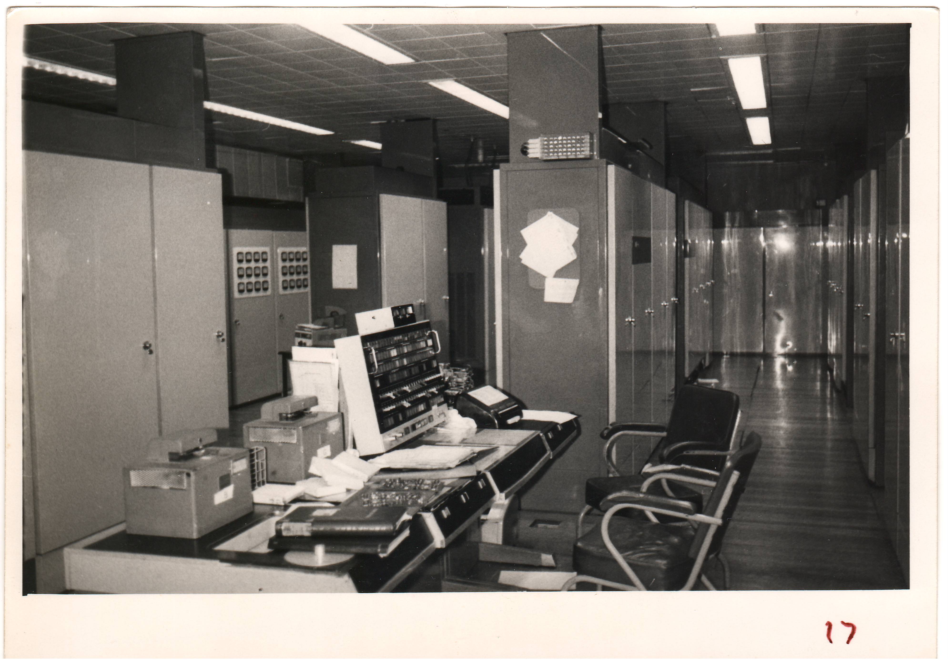
In the ATLAS hardware there were, in fact, four stores: the one-level store provided by the main core store and the four drums, a fixed store of 8K words, a private working store of 1K words and a collection of bistables and registers known as the V-store.
As indicated earlier, the whole store was addressed uniformly, the top three binary digits of the address indicating which store was being accessed. The table in diagram 6 shows the assignment of these bits to stores.
The fixed store was a read only store in which binary ones and zeros were represented by ferrite and copper slugs in a wire mesh. It was used to contain certain programs which could not be changed: these programs consisted of parts of the supervisor and code for the extracodes. This store had a very fast read time of the order of 400 nanoseconds which was exceptional for 1960 technology. The store was written by setting the ferrite and copper slugs into plastic combs and setting these into the wire mesh. This operation was performed by the aid of a computer - initially a Pegasus machine was used but later ATLAS itself was used.
The working store consisted of 1K words of magnetic core store and was absolutely addressed. This store was used as a private work area for the supervisor.
The V-store was a set of registers, device-registers-, slugs, associative tables, lock-out bits etc. which were all addressable.
Access to the working store and to the V-store was only possible when the machine was in a privileged (non-user) mode of operation.
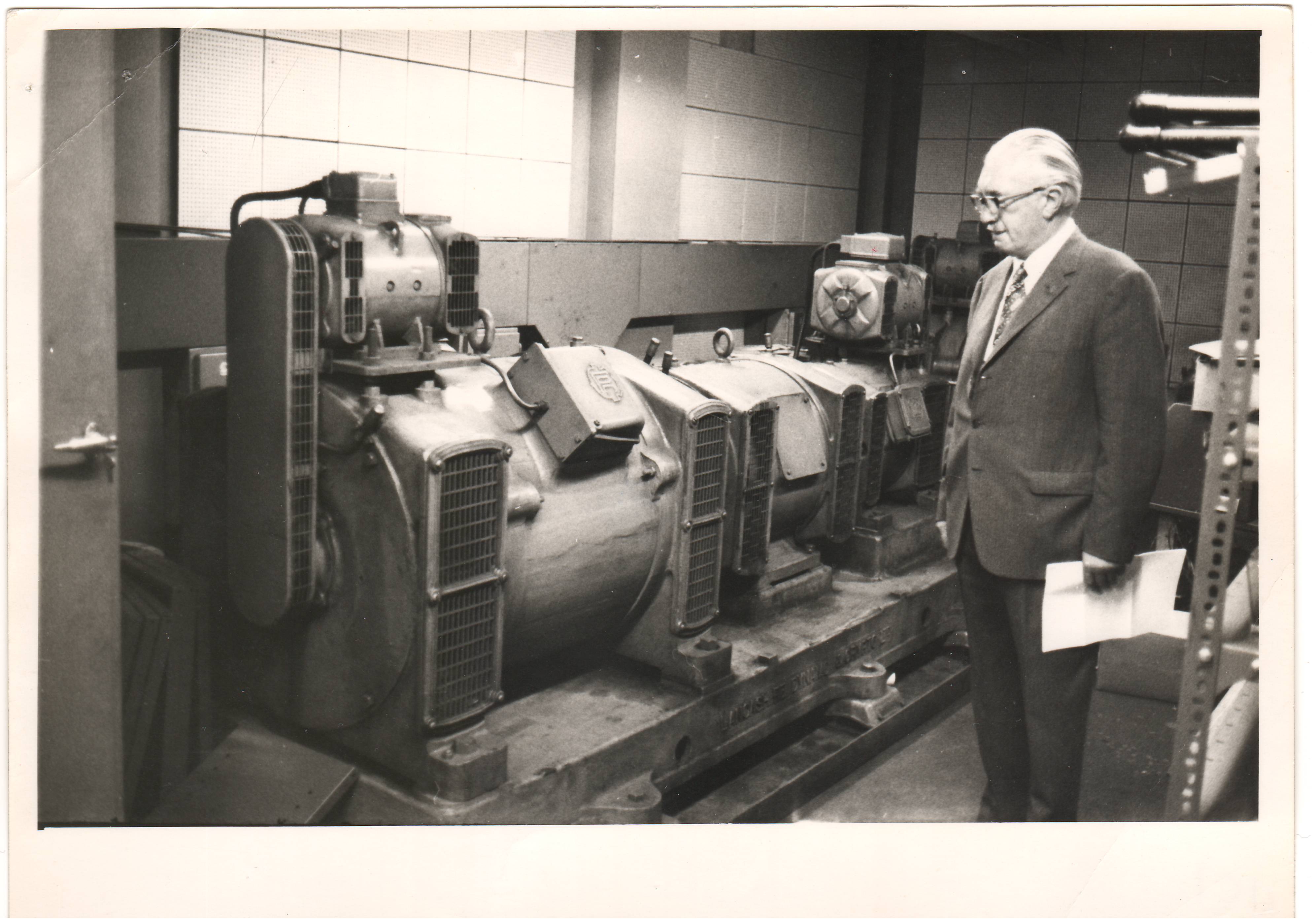
Before leaving the topic of the ATLAS store system special mention must be made of the accessing arrangements for the main core store. The core store was, in fact, arranged in stacks of 8K, each stack having its own accessing mechanism. Thus, it would be possible to access all the stacks in parallel. The core store co-ordinator unit was, in fact, responsible for arranging access to stacks in parallel. The store stacks were used in pairs, store cells with even addresses on one pair and those with odd addresses in the other pair. So, if store cell i was in pair A, then cell i + 1 and i -1 would be in pair B, and cell i -2 and cell i + 2 would be in pair A. It was then possible for adjacent words to be recovered from the core store in parallel. This is, we observe, the rudimentary principle of the interleaved store.
In this part we shall describe the sort of orders that the programmer was able to use and the view he had of the ATLAS mill. We shall also discuss how the mill of ATLAS was provided by the hardware and software.
The earlier computers usually had at least one register (or accumulator) which was used to hold the results of orders and operands for orders. Most frequently these machines had an order set with orders of the form:
Register ← register operator operand
For example, ADD R1 53
adds the contents of cell 53 to register 1, leaving the result in register 1.
ATLAS was, in fact, provided with a large set of registers, or B-lines in ATLAS terminology, one hundred and twenty eight in all, most of which could be used by the programmer. The first one hundred and twenty of these were each twenty four bits long and their arithmetic always carried out in the two's complement system. Register B0 always held zero. There was one floating point register known as the accumulator. This was made up of an eight-bit signed exponent and a double length mantissa of seventy eight bits and a sign bit. The mantissa was regarded as being divided into two parts, the most significant thirty nine bits and the sign bit known as M and the remainder known as L. The eight-bit exponent was held in the least significant part of register B124, which consisted only of nine bits.
The top bit of B124 was used to indicate whether the exponent was in range, being set to 1 when the exponent became out of range. ATLAS floating point numbers were usually held in a standardised form, the mantissa x lying in the range:
⅛ < x < 1 and -1 < x < -⅛
Yes, the exponent was held to a base eight not to the base two, so the value of an ATLAS floating-point number was given by:
sign mantissa × 8 exponent (where sign is from sign bit of mantissa )
An ATLAS store cell could be used to hold any form of information but the following formats were especially catered for in the system.
ATLAS Floating-point format: consisted of forty-eight bits, the top eight being the exponent and the other forty bits the M part of the number.
ATLAS also was specially geared to hold two twenty-four bit numbers, these usually being taken as 21 bit signed integers in the top twenty-one bits of the half word and an octal fraction in the bottom three digits.
Eight six bit characters (ATLAS internal code) could also be held in a store cell and orders were provided to handle these.
The representation of a machine code order could also be held in a store cell. This representation specified function code, two index registers and an address.
Diagram 7 summarizes the data formats of ATLAS.
We shall now go on to consider the instruction set of the machine. It will be noticed from diagram 7 that two index registers were specified in the orders (Ba (bits 10-16) and Bm (bits 17-25)). In some operations both Ba and Bm were used to provide double indexing (modification) and in others only Bm was used for indexing. Index registers are used, together with the address field (N) of an order to produce the address of the operand to be used by that order. On ATLAS the modifiers had the same format as the virtual address (i.e. the lowest three bits specified character positions), so to operate on successive locations, using a modifier register to index through, the modifier was incremented in bit 20 not in bit 23.
ATLAS was provided with a very large set of orders (the function field was ten bits wide), half being provided directly by the hardware and the remainder by extracode routines (see later): the top binary digit of the function code field distinguished between extracodes and basic hardware orders ( =1 then extracode). The basic orders were divided into three main groups:- B-codes, A-codes and test orders.
The B-codes used only the Bm field as a modifier and performed their operations on the B-line register specified in the Ba field of the order. This group consisted of the usual register operations: add, load, store, collate (i.e. AND), OR, non-equivalence, negate etc. There were also some fairly powerful test orders that would allow the contents of the Ba register to be replaced by the N field of the order depending on the Bm register being zero, nonzero, etc. A number of orders in this group also aided indexing: one for example had the effect:
If the contents of Bm are non-zero add 1 (in bit position 20) to Bm and set the N part of the order into register Ba. If the contents of Bm are zero, then leave the contents of Bm and Ba unchanged.
This order was especially useful when it is disclosed that the program counter was referred to as register B127. Also within this group are the B-test orders. The B-test register was a two-bit register and when a number was set into this register one of the digits in that register was set to indicate if the number written to the B-register was =0 or ≠0 and the other set to show if the number was ≥ 0 or < 0. Orders were provided to write a number to the B-test register and to test the above conditions, altering registers accordingly. For example, If the B-test register is set non-zero, place the N part of the order in register Ba and add 1 (at bit 20) to register Bm.
Six-bit shift orders were provided in this group: these basic shift orders were intended primarily for use in extracode routines to provide character handling and a wider variety of shift orders.
The A-code orders provided the floating point arithmetic of the computer. The operations included addition, subtraction, division, multiplication, standardising orders etc. These orders used the double modification of the machine, the floating point accumulator being implicitly used. Most of the floating point orders left the accumulator standardised and a comprehensive group of floating point test orders were included. The floating point was, of course, carried out in the basic hardware in the same way as other basic orders.
The test orders have, in fact, been mentioned already in the above two paragraphs, but it is worth making one or two points again. They had a general form of if <condition> then load register Ba with N (and optionally an operation on Bm) else do nothing. These orders were powerful enough to effect a comprehensive transfer of control mechanism because the program counter for user mode (and the other program counters too) was actually register Bl27.
(Registers Bl26 and Bl25 were the program counters for extra-code and interrupt state respectively.) Thus, a transfer of control in user-mode was simply effected by loading a value into the register B127. Conditional transfers of control were then implemented by using the test orders, and unconditional jumps by loading a value into Bl27.
At this point it seems appropriate to mention the special properties of some of the other registers. Register Bl24 has already been mentioned as holding the exponent of the floating point number in the accumulator. Register Bl23 was known as the B-log register with the special property that the value read from this was not the last value set into this register but the characteristic of the logarithm to the base two of the eight least significant digits of that number. (That is, the position of the most significant 1 bit in the last eight bits). For example, if we set the value
This register was used extensively by the supervisor in locating the cause of interrupts, and allowed this to be achieved in between two and six orders. The ordinary programmer could not use this register because of the danger of an intervening interrupt.
Registers B122 and B121 were provided with special circuitry and they allowed indirect modification of the Ba operand in an order to be achieved. B121 only consisted of seven bits and when used in conjunction with register B122 its contents were interpreted as the address of a register in the range 0 - 127. Whenever B122 was specified in the Ba field of an order, the contents of B121 were taken as a register address and the order was obeyed as if that register had appeared in the Ba field in place of B122. This pair of registers played an important part in the extracode system. Whenever an extracode was met, just before the switch was made to the extracode (see later) the Ba digits in the order were copied into B121 by the computer hardware, so allowing the extracode routines to operate on the Ba register specified by using register B122. The programmer was able to use this pair provided that he did not use any extracodes while using them, otherwise the values would be lost.
Register B120 was the engineers' console lamps and any value set into this cell appeared on those lamps: This was only useful for engineers' test programs.
The ordinary user, then, had to share his registers with the system; this did not just include the special registers but some of the ordinary B-lines. Diagram 8 gives details of those registers used by the system - the user still has a lot to use for himself.
The user was not prevented from using these registers used by the system but would probably obtain undefined results by doing so.
The basic order code was quite extensive but was extended by provision of extracodes. These were routines written in the basic instruction set which were stored in the fixed store and carried out many useful operations, some of which were (and often still are) provided only in a subroutine library. Extracodes appeared identical to other orders and were recognised by having the top bit of their function codes set to a 1. ATLAS was the first computer to include extracodes.
The programmer wrote his extracode orders in the same way as he wrote any other order, and the two types were able to be freely mixed. When the hardware detected that the order to be obeyed (i.e. the order in the order register) was an extracode by detecting that the top bit of the function code was a 1, the order was not decoded as usual, but the following action undertaken:
1 0 0 0 0 0 0 0 0 0 f1 f2 f3 0 0 f4 f5 f6 f7 f8 f9 0 0 0
Basic orders were then obeyed from the fixed store at a location deduced from the function code specified. The first order of each extracode was a jump from the entry point table to the body of the routine. The extracode routines accessed their operands by using the address in register B119 and the B121, B122 facility. The extracodes all ended with an order (f1 = f3 = 1) which when obeyed returned the control to the main control, and the order whose address was in register B127 was the next order that was obeyed, this being the order after the extracode, if the extracode had not caused a jump to have been initiated.
These routines greatly supplemented the basic order set, and no doubt helped to make programming ATLAS a lot easier.
It is worth noting that the ICL 1900 series of computers also have extracodes and these are used extensively. Every machine in the ICL 1900 range has an identical order set (as far as the programmer is concerned), but the real hardware of each member of the range is very different. Extracodes are used to provide this range standard order code. Some of the orders (floating point for example) are provided by software activated by extracodes on the smaller machines, but by hardware on the larger machines. The programmer uses these orders in the same way on both the small and larger machine. Some of the orders, the I-O orders, are carried out by extracodes on all the computers in the range. The extracode facility has allowed the range to develop maintaining a standard order set for the whole range. On the 1900 computers the extracode routines are held in the part of the core store used by Executive and not in a separate fast store as on ATLAS. No other commercial machines have yet realized the potential of extracodes.
We note again the way the hardware and software of the machine were knit together to provide the user with a virtual mill consisting of most of the real hardware plus a huge set of extracode orders to supplement this basic order set. Very few machines have ever had such a large instruction set as ATLAS had. It may be argued with some degree of justification that this was a wasteful set of orders and only very few of them were indeed ever used, and that a better set might have been chosen as the basic set to be provided by the hardware. Whatever one's personal view of the order set, at least almost everything one ever wished for was there, somewhere!
This part of the computer system is the mechanism that causes the stored program to be obeyed, and the unit which sends the control pulses to and reacts to signals from the other parts of the machine. It should be remembered from the introduction to this book that the discovery of the INTERRUPT allowed the computer to change from one task to service some event, then resume the interrupted task.
This servicing of interrupts often involves the examining of special flags and registers that the ordinary user would have no need to access, only the servicing routine need look at them.
In this sense, then, the interrupt servicing routines must be afforded some form of 'privilege' that allows them to examine registers and flags, perhaps normally forbidden from user access. Often this privilege will also include the use of some special orders (usually in connection with signals and setting flags). Most computers have, in fact, two modes of operation - the normal user mode and the mode for use by those parts of the operating system that need to examine the special registers and use the special orders. The control unit controls both modes of operation and administers the change of mode.
How will this change the way in which control operated in our simple model? After obeying each order (and at other suitable points) the control unit could see if any device was asking to be serviced or any other interrupt was registering servicing. If a request was found to be outstanding, then control would have to store away the value in the program counter somewhere, then load the program counter with the address of the interrupt handling routine and finally set the processor into privileged mode. The next order obeyed would be the first of the interrupt handling routine. If no request was outstanding, then control would continue obeying the next user order. After servicing the event, the interrupt routine would then execute a leave interrupt routine order which would have to return the computer to the exact state that it was in prior to the servicing of the interrupt. This would involve loading the program counter with the value stored away and switching the processor back to user mode. To ensure that the servicing of the interrupt did not change the state of the machine, it may be necessary for the machine's registers to be saved at the beginning of the interrupt routine and restored at the end of the routine.
ATLAS had three, not two, processor states and these were known as
The I-state was the most privileged state and this was used for only very small parts of the supervisor and in this mode of operation the one-level store was never used. The E-state was the next most privileged mode on the machine and it was in this mode that much of the supervisor and all the extracodes were obeyed. User programs always ran in M-state, except, of course, for the execution of extracodes they initiated.
The ATLAS control unit had two special bistables which were used to indicate the processor state, one indicating either I-state or M/E-state and the other indicating either M-state or E-state. As has already been noted, ATLAS had three and not one program counter - one for each of the three machine states. So, conceptually, at least, when obeying program, control examined the state bistables and used the appropriate program counter. On sensing an interrupt request the ATLAS hardware proceeded as follows:
Execution then continued at the order whose address was in B125. We notice that ATLAS only inhibited further interrupts when actually entering I-state; once in I-state further interrupts only set flags and did not cause a re-entry to be made to the servicing routines.
How did the service routine locate the cause of the interrupt request? Well, on many machines this is only found by examining a set of individual flags and finding the first one set, then taking the appropriate action.
All this testing would need to be performed by orders and could be quite a lengthy process. On ATLAS there were about one hundred different reasons for an interrupt occurring and such a software method described above would have been far too slow.
Here again, we observe the way in which the hardware and the needs of the operating system have been married together. The device flags (these were one-bit indicators which were set whenever the device or event they represented required servicing) were built up into a tree structure consisting of four levels. At the lowest level of this tree were the device flags, and these were grouped together in eight-bit registers. Each level of the tree was connected to the next highest in such a manner that the groups of eight bits at the lower level were connected to one bit at the higher level. At the root of the tree was a single bit indicator known as the Look At Me (LAM) bistable. These flags and registers were all part of the V-store. So, for example, if a tape reader wanted servicing, it would set its own device flag in the lowest level of the tree and so set the tape reader bits all the way to the top of the tree setting the LAM bistable. The setting of this flag informed control that an interrupt required servicing.
Diagram 9 illustrates a simplified version of part of the interrupt tree.
To discover the cause of an interrupt, programmed orders (held in the fixed store) were used in conjunction with the B-log register, B123. The top level of the tree was loaded into B123 (giving the position of the most significant 1 in this level): a jump was made using the value in B123 as a modifier. This sort of action was repeated, loading the registers for levels into B123 as appropriate, then jumping.
This system very rapidly located the cause of the interrupt. The supervisor's interrupt routines were all kept very short and most of the servicing routines only took the minimum amount of action, causing a request for the appropriate SER to be run. (See later)
At the end of each interrupt routine the control was transferred to the beginning again to check for any further interrupt requests to allow these to be dealt with. If no interrupts required servicing the exit from the interrupt servicing was performed. This simply involved setting the I/ME bistable back to the ME state. Control would then continue obeying orders from the specified cells in either B126 or B127 depending on the machine being in E-state or M-state.
The observant reader will have noticed that ATLAS did not, in fact, change registers, so that values in some of them will have been changed. It will be remembered that the registers were partitioned between the user and the system providing a simple and fast solution.
The high speed of interrupt entry and exit is very largely due to the very specialized hardware used in the computer, and indeed, I believe that the entire interrupt system shows a very well engineered overall system with full hard and software integration.
The method used to search the interrupt tree for the demanding device/event imposed a priority on the order in which the supervisor serviced the interrupts. This priority is imposed by the method used to search the tree and in the way the device flags were allocated within the tree. The priority was used by the designers to ensure that those devices that had to be serviced fast were serviced first. (The original paper tape readers were like this, as they would lose a character if it were not taken directly from them.) The order of priority was roughly: parity failures, magnetic tape peripherals, card readers, paper tape readers and punches, line printers, non-equivalence (from the one-level store), drum events, division overflow and illegal function codes. It will be noticed that extracodes were obeyed in a special mode, E-state. The entry to and exit from extracodes has already been dealt with in the section on the Mill. Extracodes like ordinary user programs could be interrupted.
The control unit of ATLAS was also concerned with operating a simple instruction pipe-line. This was again an idea pioneered in ATLAS (and in the IBM STRETCH machine) and is one of the topics of great current interest. Essentially pipe-lining involves the overlap of parts of one order with others. For example, while obeying one order, there is no real reason why the next one to be obeyed is not obtained from the store, and while actually reading from the store, the program counter may be incremented. This is by no means a simple sort of system to try and implement. The reader should be aware that this currently fashionable idea was pioneered some time ago.
Most computers have an extensive set of input-output peripherals and ATLAS was no exception. The LONDON ATLAS peripherals consisted of:-
All the slow peripherals (that is all except the magnetic tape units) were controlled by the peripheral co-ordinator, and had device buffer registers and flags in the V-store. The supervisor actually managed all of these devices and these slow devices were never driven on-line by a program other than by the supervisor. The huge difference in speed between the central computer and these devices would have made it economical suicide to allow these to be driven directly by a program.
The virtual peripherals seen by the ATLAS user fell into two types - the slow peripherals and the fast peripherals. The fast peripherals consisted essentially of the magnetic tape units and these are described in a later section. The slow peripherals were, in fact, spooled by the supervisor onto a magnetic tape. For example, if the user wanted to read a paper tape in his program, the supervisor would first read the paper tape in and store it on a magnetic tape known as the system input tape When the job requiring this tape was being processed, it would input its data by using an extracode which would initiate supervisor action to provide the data which it had spooled away. (See later for details.) The user in fact, was only aware of a set of logical device streams and the actual devices that supplied the information only of interest to the supervisor. All input and output via the slow peripherals was converted to (from) a standard internal code, known as the ATLAS Internal Character code. Every document read by file system was transferred into this code, unless specified as binary. This facility allowed various external representations to be used, and the user merely informed the system what external code had been used and the part of the supervisor that read the documents carried out the appropriate translation. This greatly aided making program devices independent.
Extracode orders were provided to deal with these logical devices: the programmer could select a logical channel, read characters or records from it, write characters or records to it, etc.
The user's virtual slow peripherals were indeed very simple to use (as easy as in high-level languages) and that's how they should be in all systems!
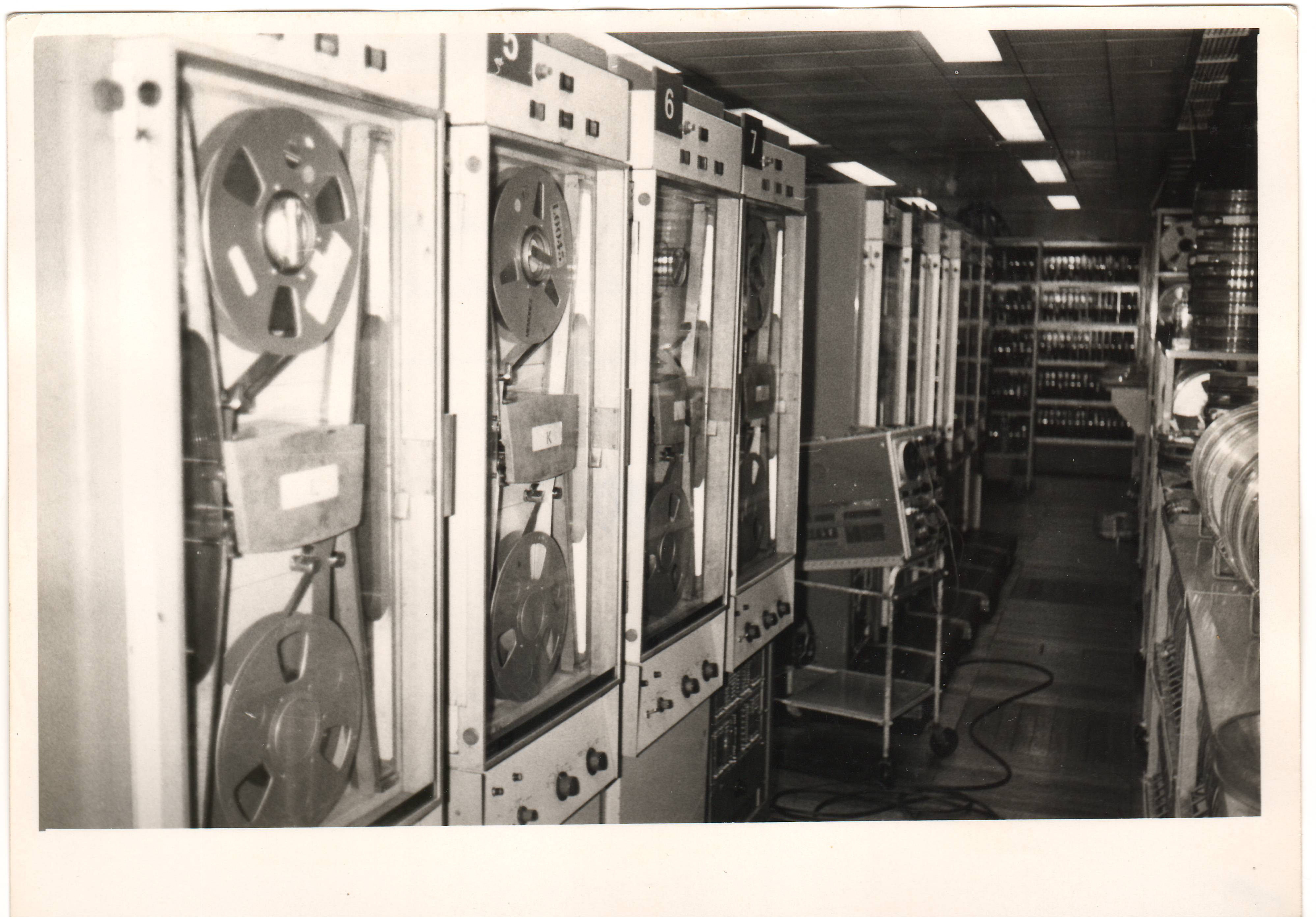
The ATLAS ONE INCH MAGNETIC TAPE SYSTEM was of a very special type. A normal magnetic tape system allows data to be written to or read from the tape in a serial fashion only during one pass over the whole tape. Thus, to update a file on such a tape, it is necessary to copy the whole tape from start to finish incorporating the appropriate changes in the new version. The ATLAS One Inch Tape System was rather cleverer than this. Every magnetic tape, before being brought into use was initialized with blocks and block addresses. The tape decks and their controllers were specially designed so that the tape on the deck could be positioned at a specified block, enabling any named block on the tape to be accessed. This tape system, then, allowed the initialized magnetic tapes to be used in a random fashion, allowing the addressed block to be either read or written. This facility allowed the updating of individual blocks within a magnetic tape without the need for copying the whole tape. Although random access was possible with these tape decks, it was rarely used as the latency time was very high perhaps as long as 3 - 4 minutes. Extracodes were provided for the users to read and write blocks into these tapes: there were also extracodes to title a tape and request that a tape be mounted. These tapes were, of course, intended for binary output. The One Inch Tape System was essential to the operation of the ATLAS supervisor, three such decks being needed. One was used for the system input tape, one for the output tape (the spooling) and one for the supervisor itself. This last unit held the most commonly used compilers as well as the supervisor. This tape system proved to be rather less reliable than it had been hoped it would be and must be regarded as one of the reasons the system never reached its predicted performance.
Having now described each of the units of ATLAS, we shall now think about the way the user actually used this virtual processor, and how the supervisor went about organising things.
With hands-on access to a machine, the user could simply input his program directly, then make the system (if any) obey him by typing commands or setting hand keys. This is also true of an interactive system. ATLAS provided a batch service, not an interactive system, forcing the user to supply, in addition to his program and data, instruction as to how his job was to run. Because ATLAS was substantially an automatic batch system, run without operator intervention, the instructions on how to run the job were given to the supervisor program.
ATLAS had a fairly simple, though quite comprehensive, job control language. The user simply submitted his program, data and job control documents, each on any media he desired, and his job was run. The term document in ATLAS terminology had the special meaning that it was a self-contained section of information presented to the computer through one input channel. For example, a collection of data on a length of paper tape was a document. Each document carried at its head a heading and a title and an end of document mark at its tail. As each document was input, the supervisor would put the document on a list which gave the type of document and the place on the input tape where it had been stored.
The document with the heading JOB was the document that contained the instructions to the computer telling how a job was to be run, and was known as the job description. The line after the heading gave the title of the document, and this was the name used by the supervisor for that document. The job description gave full details of all other documents needed to execute the job, together with estimates of store and time required. There was no concept of the job step (as in OS/360 on George 3) in the ATLAS job description, only one step could be specified per job description. This was a disadvantage, forcing multi-step jobs to be run as many small jobs.
The document headed COMPILER was known to hold the source of a program to be compiled using the named compiler. The heading DATA said that the document following was to be used for data. Diagram 10 shows an example of an ATLAS job.
Let us now consider the way the user's job was run by the ATLAS supervisor.
The various documents for the job were input through the computer's peripherals - each document could happily be on different media - and stored away on the system input tape by the supervisor. The supervisor recorded the name, type and location on the input tape of each document it received. Once all the documents for a particular job had been read in, the job was put onto a private list of the supervisor's, known as the job list which held jobs that could be run. Every job on the job list was classified into one of eight groups according to its attributes. These groups divided the jobs principally into high priority job, tape job, short jobs, long non-tape jobs and low priority jobs. The scheduling part of the supervisor then selected jobs from this list and put them onto the active list, removing them from the job list. Once on this list, the job control document for the job was read from the system's input tape and a coded form of this set up. The supervisor then requested the operators to set up any magnetic tapes required by the job. Communication from the supervisor to the operators was handled over one of the teleprinters. To communicate with the supervisor, the operators originally had to input a message through any one of the slow peripherals, as the machine had no teletype-like device communications had to be carried out by means of paper tape or cards. (A typewriter was added to the London ATLAS during its life.) This, however, was not as serious a drawback as it would appear to those familiar with the IBM 360 or ICL 1900 computers. The ATLAS supervisor was a very advanced and sophisticated piece of program and needed very little information from the human operators, that even when fitted, the console typewriter was of very little use.
The supervisor merely issued requests for the operators to act upon. It would request for magnetic tapes to be mounted, printer paper to be reloaded, etc. You may wonder how the supervisor was told as to which tape was mounted on which deck - well, the answer is simply, it wasn't! The supervisor found this information out for itself by reading the tape number from the magnetic tape: once the operator mounted a tape, he pressed the engage control which signalled the supervisor to identify the tape. This certainly made the mounting of the wrong tape rather more difficult.
Once all the tapes required by the job were mounted, the supervisor would then read the first few blocks of each input document required by the job from the system's input tape into its INPUT WELL and a copy of the required compiler was recovered from the supervisor tape. The INPUT WELL was an area of the store where the supervisor held buffers for each active job: in reading data into a job, the supervisor would hand the data from the system's input tape into the INPUT WELL, then hand it over from there to the program. A similar arrangement existed for the output. Diagram 11 shows the total arrangement of the ATLAS spooling system.
Once all the above had occurred, the job was moved onto the execute list. From this list, the completely assembled jobs were selected by part of the supervisor known as the execute scheduler and multi-programmed together. Output was written from the jobs via the SYSTEM OUTPUT WELL onto the system's output tape. Once all the output for the job had been converted to hard copy, the input and output documents were removed by the supervisor from the system input and output tapes.
One notices at once how little human intervention ever occurred in the processing of a job - the operators appear only to serve some primeval god, feeding it with information in response to its commands. The size of the lists used in the system were kept fairly small so that there was never more than twenty-four jobs in the machine at once: once this limit was reached, the machine refused to eat any more. The restriction on the number of jobs in the machine at the same time was partly due to the failure of the magnetic tape system in meeting its predicted performance, making the Input and Output tapes less reliable than was needed.
So far, we have only mentioned the supervisor as performing tasks. Let us just peep at the sort of beast this remarkable piece of software was.
The supervisor controlled all the system functions not provided directly in the hardware of the machine and dealt with organising and running the entire machine's resources. It was activated in many ways - as the result of some user program requesting a peripheral transfer, as the result of a one-level store transfer being necessary, and as the result of an interrupt.
The ATLAS supervisor consisted of many different routines which were normally dormant but which could be woken up when required. These routines were known as Supervisor Extracode Routines (SERs). All the supervisor's tasks were carried out by SERs, these being obeyed in E-state and many of them residing in the fixed store. The SER's not in the fixed store were held in parts of the one-level store owned by the supervisor. The SERs were activated as the result of some form of supervisor request being made and their activation was achieved via a special routine known as the co-ordinator, which arranged a priority of execution for the SERs.
Because SERs were written to be obeyed in E-state, they could be interrupted by interrupt requests.
The supervisor was, in fact, held on the supervisor magnetic tape with parts loaded into the one-level store. The most used SERs were permanently set in the fixed store. Because some programs existed permanently in the machine, this meant that starting was relatively simple. Once the machine had been powered up, it only needed the relevant fixed store routine to be entered, to load the rest of the system - this was achieved by pressing the engineers' interrupt control. Essentially, this caused some basic hardware tests (also stored in the fixed store to be executed) and then the supervisor to be read down from tape into the store - a lot easier than loading a bootstrap via the hand keys.
Although development was initially very slow, ATLAS eventually was well endowed with an extensive set of compilers and utilities. In this section we shall give a survey of some of these.
The list was long, but included the following:-
          ABL
          FORTRAN V
          HARTRAN
          ATLAS AUTOCODE
          ALGOL 60
          COMPILER-COMPILER
          BCL
          MERCURY AUTOCODE
          SERVICE
          EXCLF
         COPYTAPE
The ABL Compiler (ATLAS Basic Language) provided a convenient, simple way of assembling machine code programs. Each ABL instruction corresponded to exactly one machine order (basic or extracode order) and each part of the ABL order mapped exactly on to the corresponding parts of the machine instruction. In its simplest form, an ABL order consisted of four numbers corresponding to each part of a machine code order, but extensive facilities were provided for the user to use a wide variety of symbolic expressions. A full set of system directives were also provided to allow the complete assembly of programs and a library of routines was provided.
The HARTRAN compiler was the first ATLAS FORTRAN compiler, and was developed for the Harwell ATLAS and included many useful extensions to that language.
The FORTRAN V language was developed by Atlas Computing Services in London and provided ever more powerful extensions to the language than HARTRAN had. The extensions in FORTRAN V included a block structure, fully dynamic array, a clear statement, improved loop and format specifications etc. FORTRAN V contained A.S.A. FORTRAN IV as a subset and was quite compatible with IBM 360 FORTRAN and HARTRAN.
The ATLAS ALGOL 60 system provided a fairly flexible system, allowing many different representations of ALGOL 60 to be used. Simple I/O procedures were provided and the user had the option of selecting his routines from libraries that were compatible with many other computers including the KDF9 and ICL 1900 machines.
The compiler known as COMPILER-COMPILER was designed by R.A. Brooker and D. Morris especially to aid the compiler writers in writing the set of systems compilers for ATLAS at Manchester. Compiler-Compiler language was specially orientated towards the writing of compilers having special facilities for recognition of phrases and for dealing with such structures.
Compiler SERVICE was, in fact, a set of system utilities and the source program for this compiler consisted of requests for various utility tasks to be carried out. These included tape dumping, copying, media converts, editing, etc.
We have now dealt with all the notable features of ATLAS, and the most revolutionary parts of the machine have been discussed. The impact of these ideas has been great on the computing world, yet still many of the wonderful ideas used in the machine have been ignored. ATLAS stands alone as a supreme example of close co-operation between industry and a university and perhaps is symbolic of Great Britain in the early 1960's.
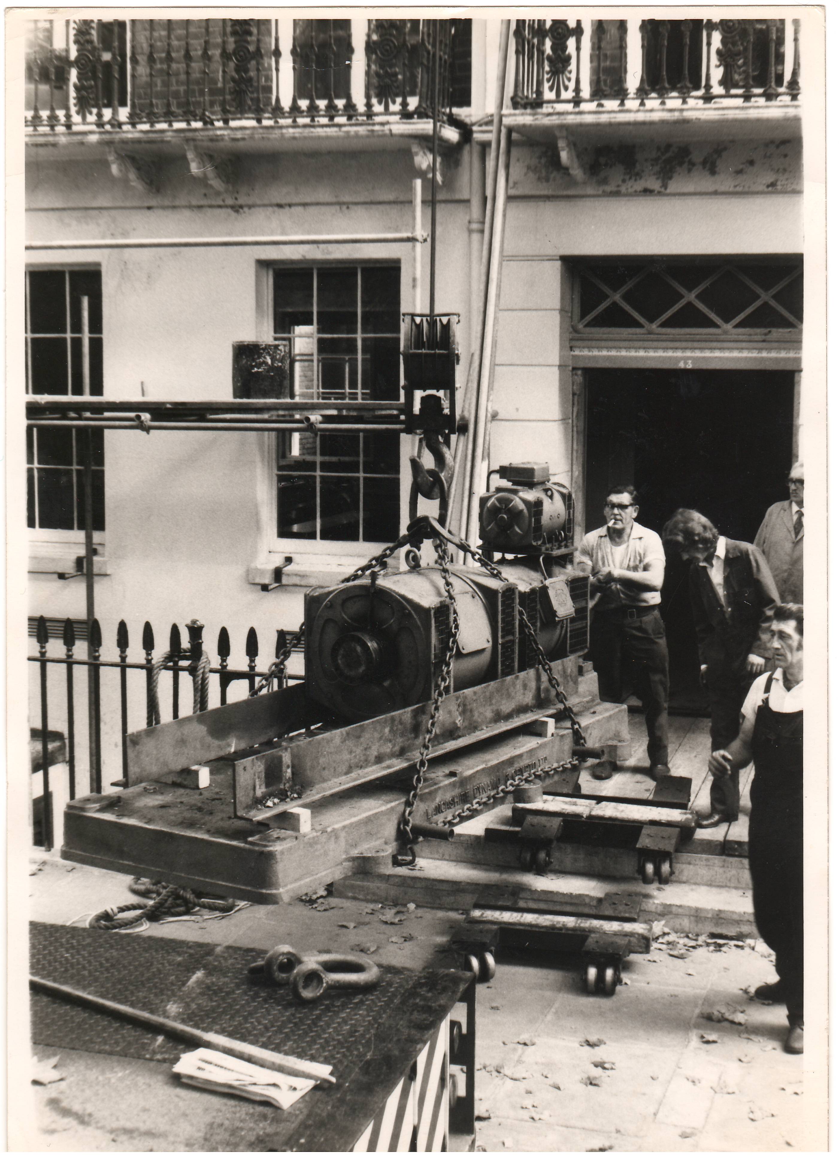
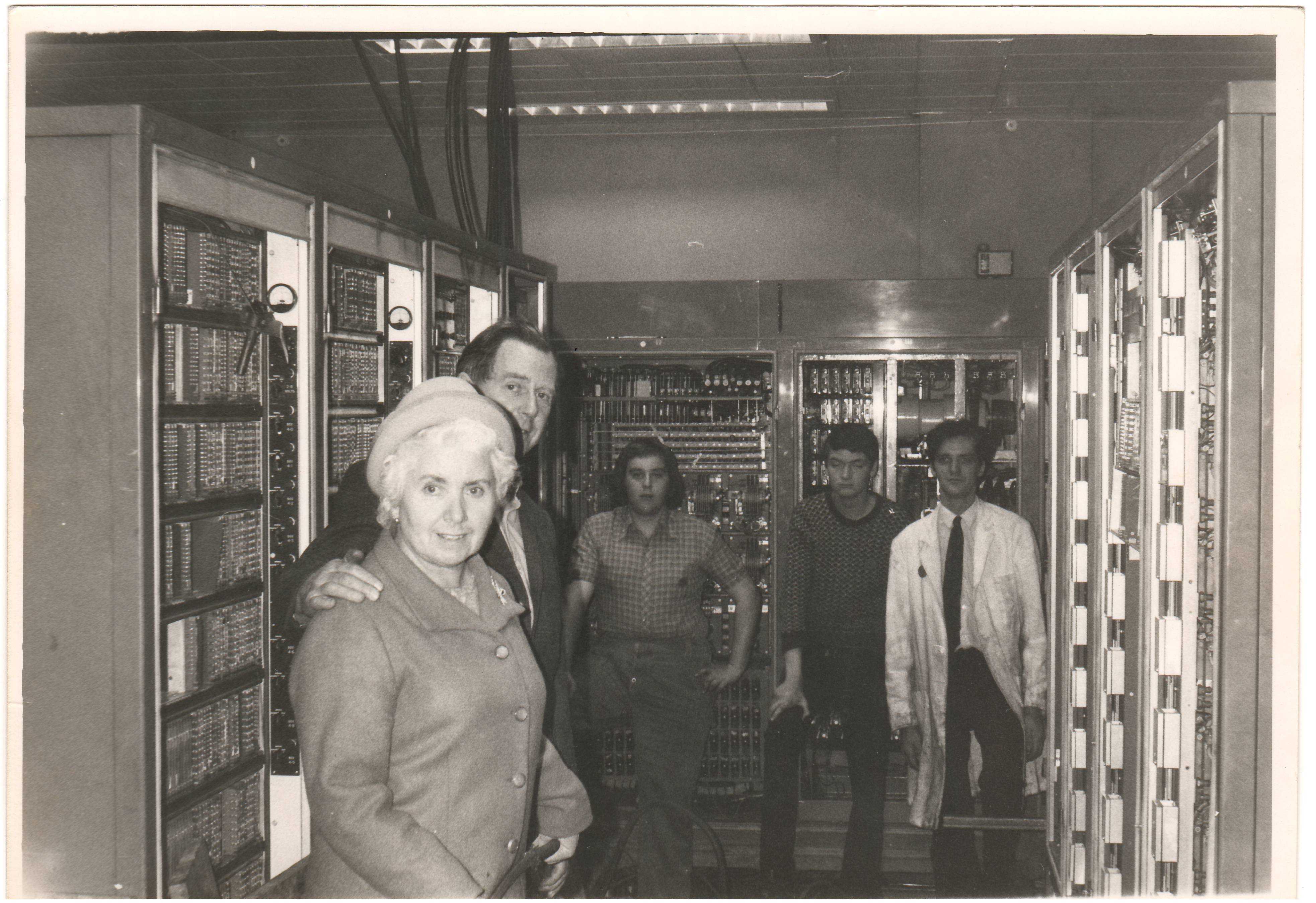
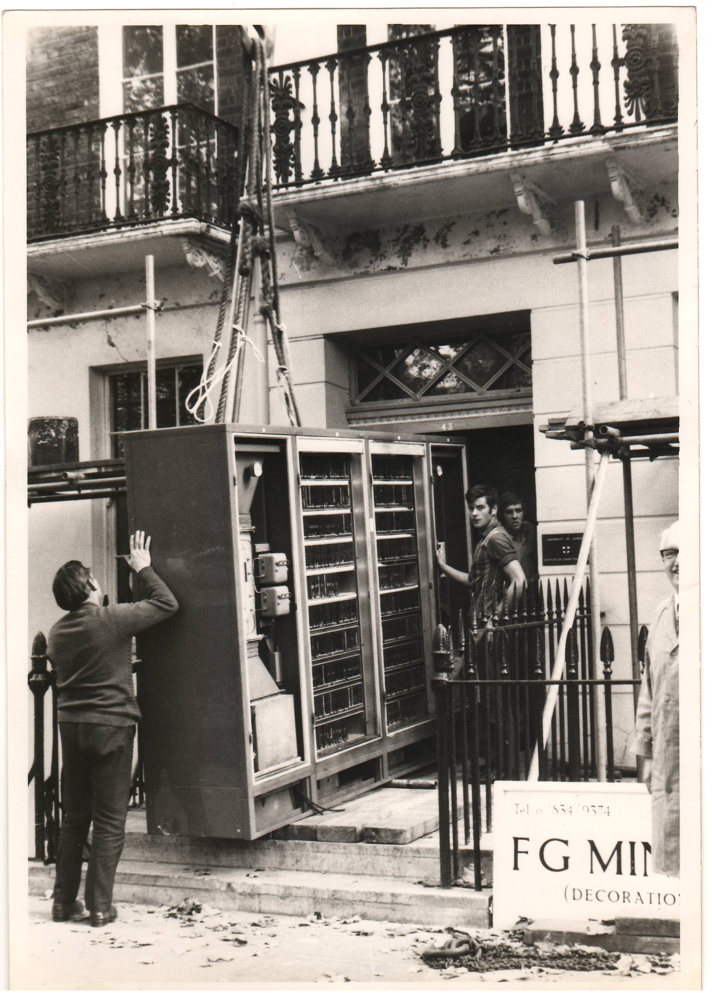
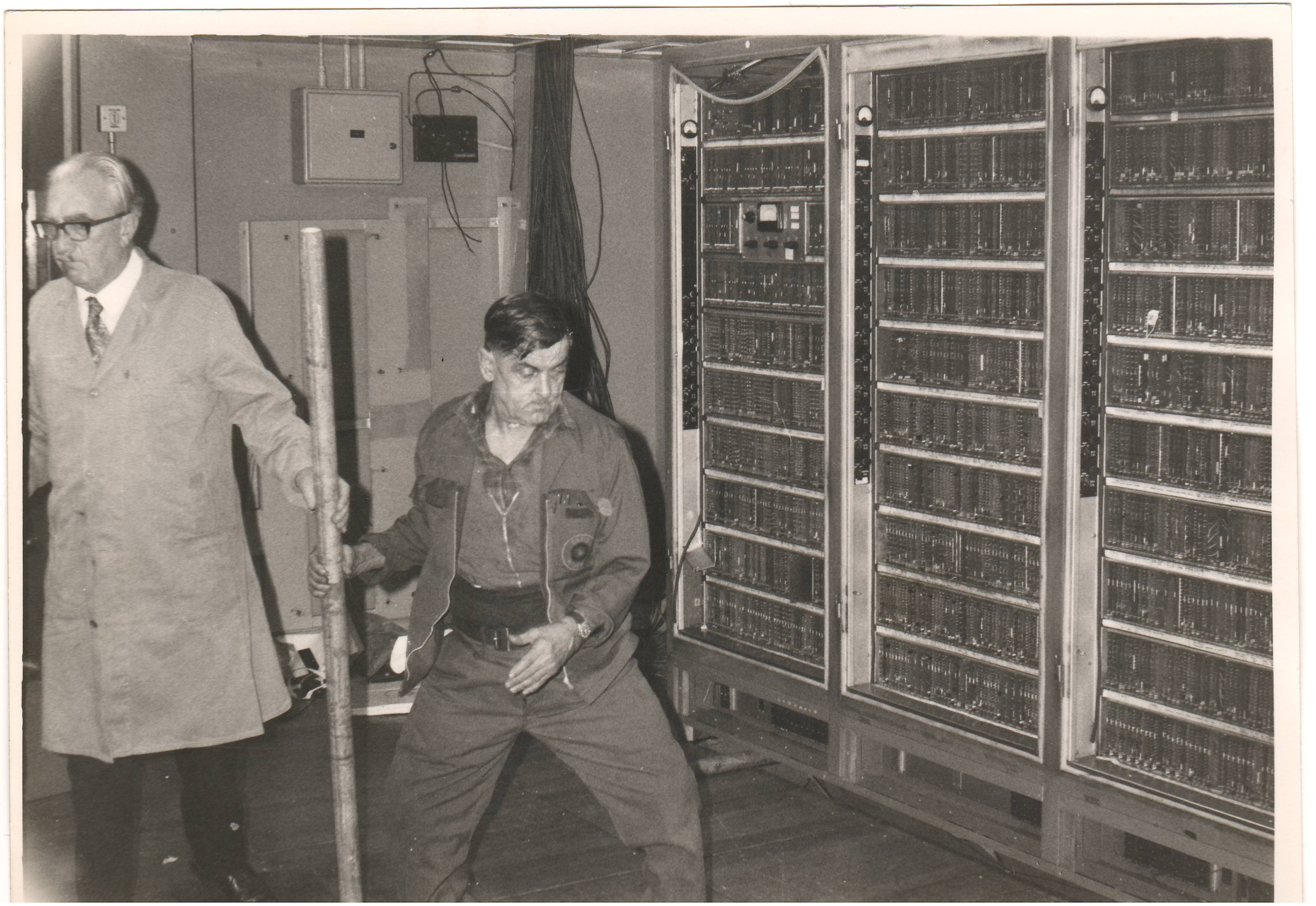
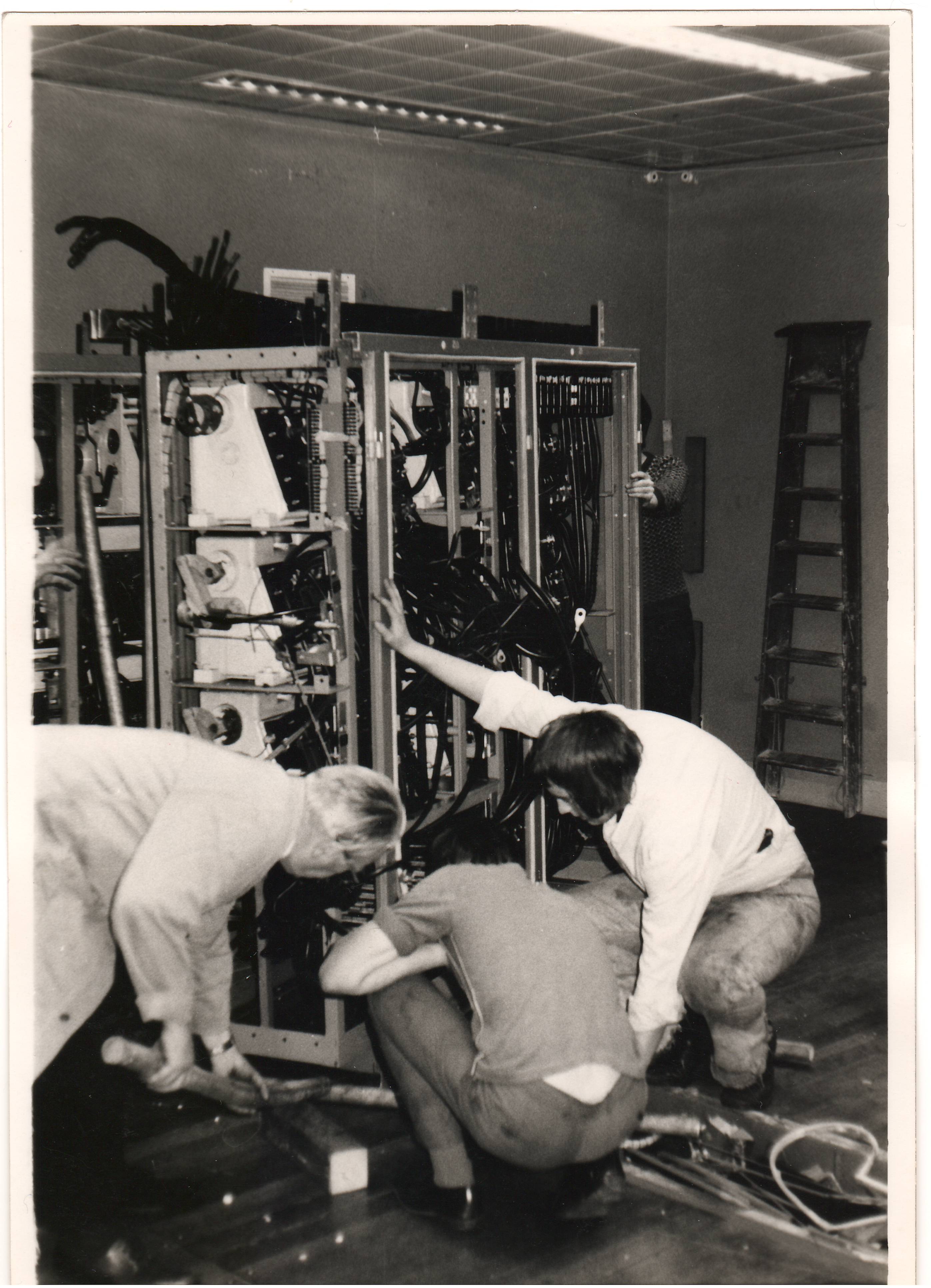
The London ATLAS and the Manchester ATLAS have now both been scrapped: the Harwell machine is shortly to follow them later this year.
ATLAS has returned, leaving the heavens to support themselves, to its place in mythology, like its fellows, Mercury, Sirius, Pegasus and Orion, before it.
1. The I.C.T. ATLAS 1 Computer: Programming Manual for ATLAS BASIC LANGUAGE (Jan. '65, List CS 348A)
2. I.C.T. Features and Facilities of ABL for the ATLAS 1 System ( June '65, List TL812
3. I.C.T. Preparing a Complete Program for Atlas 1 (March '66, C5460)
4. The I.C.T. ATLAS 1 COMPUTER The ATLAS 1 Supervisor Operating System and Scheduling System (Nov. '66, TL1685) (This is based on the four papers following)
5. Kilburn, Payne and Howarth, The ATLAS Supervisor, from "Computers - Key to Total Systems Control" published by the American Federation of Information Processing Societies
6. Kilburn, Howarth, Payne and Sumner "The Manchester University ATLAS Operating System Part 1: Internal Organisation" Computer Journal Vol. 4, No. 3, 1961
7 Howarth, Payne and Sumner, The Manchester University ATLAS Operating System Part 2: User's Description, Computer Journal Vol. 4, No. 3, 1961.
8 Howarth, Jones and Wyld, The ATLAS Scheduling system, Computer Journal Vol. 5, No. 5, 1962.
9. Ferranti Orion Ferranti 1959, List DG 40 System
10. An Introduction to Ferranti, 1956, List DC 22 the Ferranti Mercury Computer
11. Kilburn, Edwards, Lanigan and Sumner, One-level Storage System, IRE Transactions on Electronic computers Vol. EC-11, No. 2, April 1962.
12. University of London ATLAS Computing Service. FORTRAN V Manual
13. Brooker, Morris "An Assembly Program for a Phase Structure Language" Computer Journal Vol. 3, No. 3, 1962.
14. University of London Institute of Computer Science "Petit Bleu" Nos. 1 to 6 (an internal news letter for I.C.S.)
15. Financial Times 27th May 1964
