
The planets in our solar system possess many interesting differences that have fascinated visual astronomers for many years, and provoked them into providing many theories to explain these features. For example, the terrestrial planets have differing amounts of cloud cover; the Earth has 50%, while Venus has 100% and Mars has no clouds at all. On the other hand, beyond the asteroid belt lie the giant planets Jupiter, Saturn, Uranus and Neptune, their 29 satellites, and in addition, Pluto, a small planet which is more like a satellite than any of its giant companions. These giant planets contain more than 99% of the planetary mass and 98% of the angular momentum in the solar system, including the sun. One of primary constraints upon any theory of the origin and development of the solar system is the necessity of logically explaining the extreme differences between these giant planets and the terrestrial planets.
The lower atmosphere of a planet is a particularly important part of the atmosphere from the point of view of radiative transfer. It is a meteorological region; a region concerned only with thermodynamic equilibrium, where in the case of Venus and the Jovian planets, clouds present a substantial source of opacity. Furthermore, it is a source of chemical species, an anchor for upper atmosphere temperature. It provides the source of dynamical energy and thermal radiation environment for the outer layers. On Earth, this region extends to approximately 25 km above the surface, while on Venus, it extends to about 100 km above the surface of the planet. For the outer planets, we have no idea of the extent of their respective tropospheres, since at this time it is not known whether solid surfaces even exist for these planets.
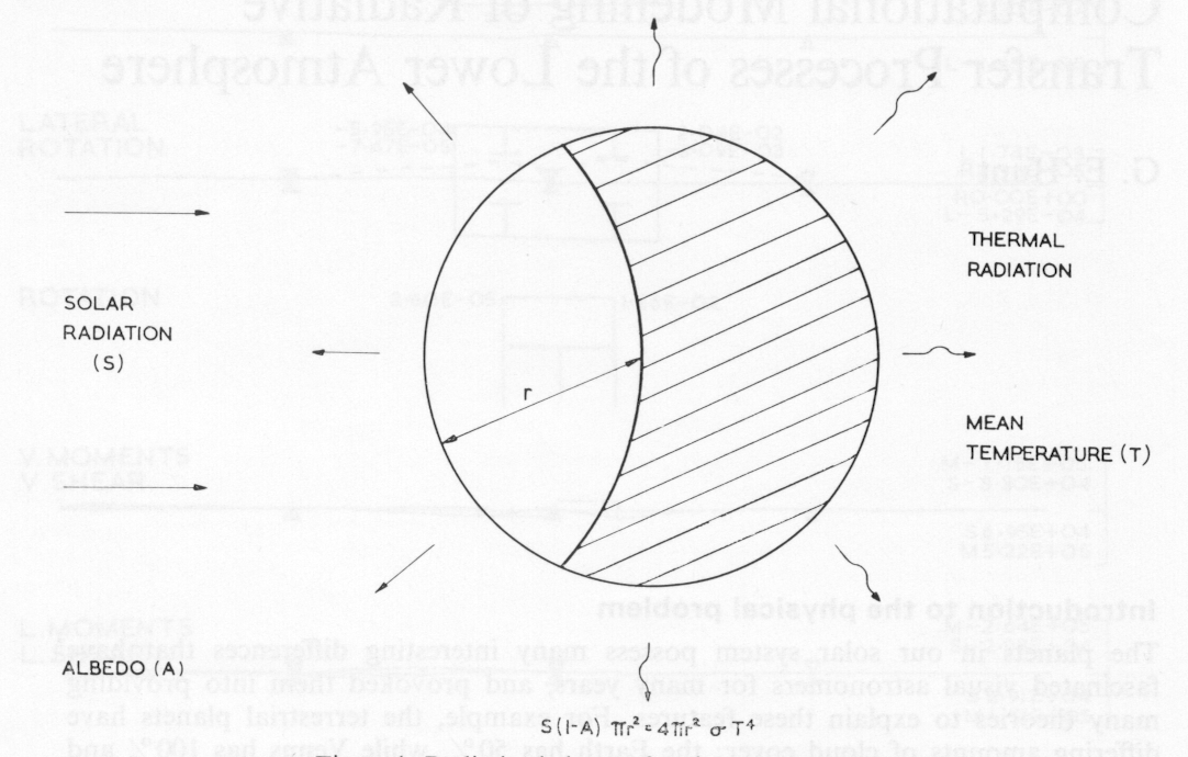
In order to understand in a simple way the planet-atmosphere system, we may imagine it as a huge thermodynamic engine with the solar radiation as the source of energy. If we then equate the total energy received by the planet to the energy lost by long wave radiation from the surface and the atmosphere (which is assumed to be at a mean temperature of T° K), we may write mathematically,
S π r2(1-A) = 4πr2ρT4 (1)
The radius of the planet is r and the factor (1-A) allows for a fraction A (the albedo of the planet) of the total incident radiation to be reflected into space from clouds and the surface. This equation, which is also shown schematically in Figure 1, is a mathematical statement of Stefan's Law (see Goody (1)), and we may apply it to any planet on the assumption that it emits radiation as a black body of mean temperature T°K. For the Earth, which has an albedo of 0.35, and using the known values of S and σ (Stefan's constant) it is easy to derive a value of 250°K for the effective temperature, which is in agreement with observations. Similarly, we have agreement between the predicted and observed temperatures for the other terrestrial planets. For Jupiter and Saturn, it appears at present, that we do not have radiation ba1ance, since these planets appear to emit considerably more energy than they receive from the sun, which suggests that they must have an internal heat source. Insufficient information is at present available about the radiative properties of the other outer planets, to know whether or not they have internal heat sources. However, this information may be readily obtained from the proposed Grand Tour Mission to the Outer P1anets or any orbiting mission to these individual planets, and it will indeed form one of the most important radiation experiments.
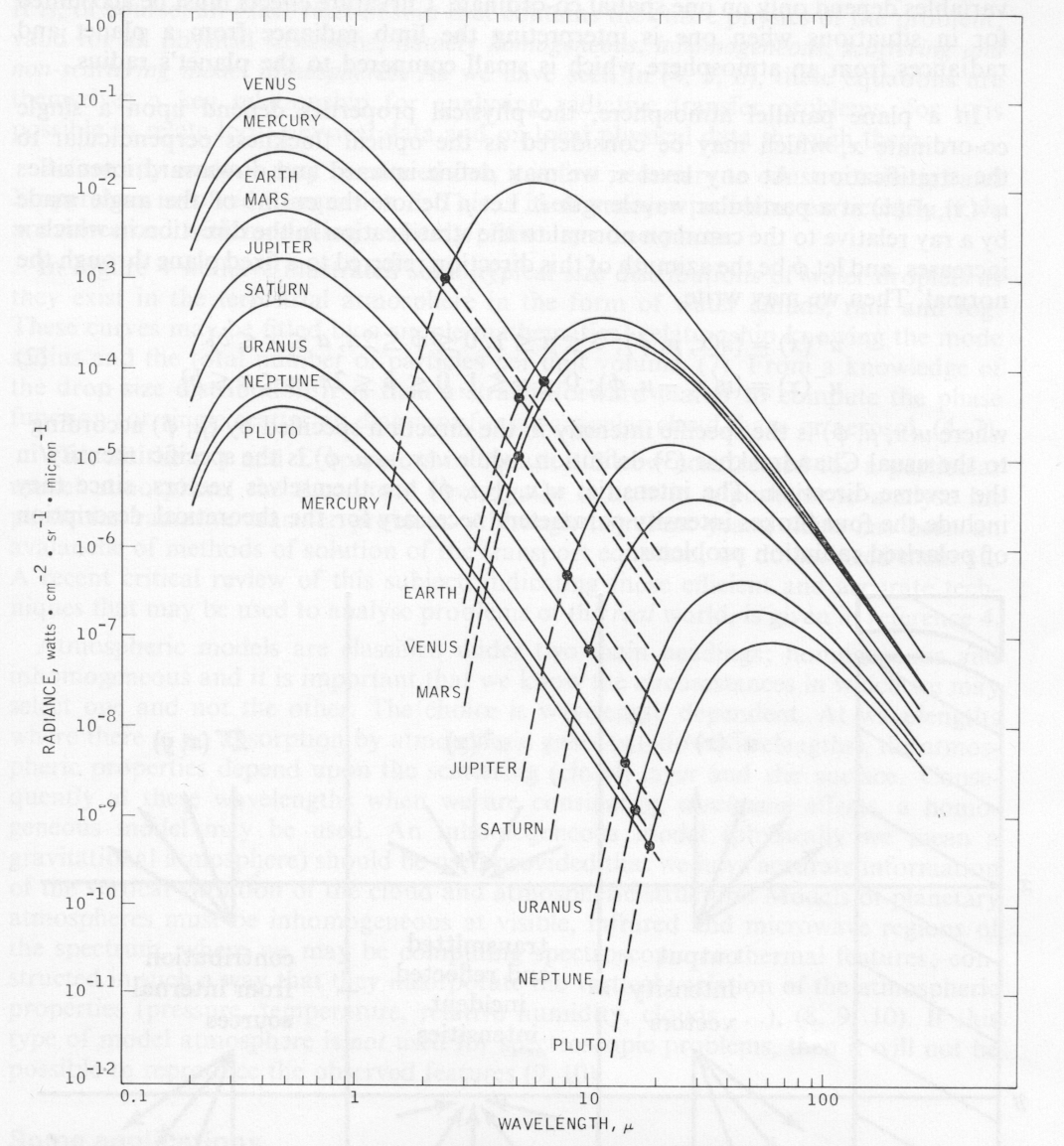
The planets receive virtually all their energy from the sun in the form of electromagnetic radiation which is emitted continuously and in all directions. The spectrum is usually divided into a number of sub intervals; the ultra violet region covers 0.25-0.4μ the visible portion is 0.4-0.7μ the near infra red is 0.7-4μ and the infra red is 4μ-1 mm. The remainder of the radiation is then at longer wavelengths (radio waves) and at those wavelengths shorter than the ultra violet (gamma rays and X rays).
The emitted thermal radiation from a planet is defined by the effective brightness temperature of the atmosphere or surface. In the case of a planet having a cloud free atmosphere, such as Mars, the observed temperature is effectively that of the surface material. For planets with extensive cloud cover the observed brightness temperature is that of the atmosphere at a level which in general, is close to the top of the visible cloud deck. At high spatial resolution the thermal region begins to show structure resulting from the variations in optical depth with wavelength characterised by the absorption spectra of the constituent atmospheric species. The spectral features can appear in emission or absorption, superimposed on the general brightness continuum depending upon the detailed thermal structure of the atmosphere. It is only in very recent years that the technology has reached a point where this spectral structure can be measured quantitatively with precision necessary for its interpretation of vertical temperature structure (see for example Houghton and Smith (2)).
The shorter infra red wavelengths which reach a peak in the visible range define the solar reflected radiation as we have previously pointed out. The intensity of the reflected component is controlled by the albedo of the planet; the reflectivity of the surface in the case of the transparent atmosphere, or the spherical albedo of the cloud layer. The spectrum is observed in absorption, the absorption features being characteristic of the fundamental, overtone or combination vibration-rotation bands of the constituent atmospheric molecules, superimposed on the solar continuum.
It is possible to treat the solar reflected energy and the thermally reflected energy from an atmosphere, separately. If we take the Earth as an example, we find that at a temperature of 250°K, the radiation of wavelengths less than about 4μ is of negligible energy, while the solar flux carries little energy beyond this wavelength. Consequently, for the Earth, the division between reflected and emitted energy occurs at around 4μ. In Figure 2 we have shown schematically the spectral characteristics for the planets, and it is apparent from this diagram that the wavelength corresponding to the division between solar and thermal fields increases in magnitude as the effective temperature of the planet decreases.
It is apparent from what we have stated here that the interaction of electro-magnetic radiation with the gaseous, particulate constituents and cloud particles of a planet's atmosphere is an extremely complicated process. Consequently the interpretation of the radiation field emerging from the atmosphere, to derive the atmospheric structure, composition and cloud properties forms one of the fundamental problems of atmospheric physics.
A great deal may be learnt from computational models of a planetary atmosphere since the physical processes which describe the interaction of the radiation field with the cloud particles are well known (1). Theoretical work of this type is also extremely important from the point of view of designing instrument packages and scheduling observational programs.
The majority of problems that concern us in atmospheric radiation have the simplest geometric configuration, that of a plane parallel atmosphere so that the physical variables depend only on one spatial co-ordinate. Curvature effects must be accounted for in situations when one is interpreting the limb radiance from a planet and radiances from an atmosphere which is small compared to the planet's radius.
In a plane parallel atmosphere, the physical properties depend upon a single co-ordinate x, which may be considered as the optical thickness perpendicular to the stratification. At any level x, we may define upward and downward intensities u+(x),u-(x) at a particular wavelength λ. Let μ denote the cosine of the angle made by a ray relative to the common normal to the stratification in the direction in which x increases and let φ be the azimuth of this direction referred to a fixed plane through the normal. Then we may write,
u+(x) = {u(x, μ, φ); 0 ≤ μ ≤ 1, 0 ≤ φ ≤ 2π, a ≤x ≤ b}
u-(x) = {u(x, -μ, φ); 0 ≤ μ ≤ 1, 0 ≤ φ ≤ 2π, a ≤x ≤ b}
where u(x, μ, φ) is the specific intensity in the direction specified by (μ, φ) according to the usual Chandraskhar (3) definition, while u(x, -μ, φ) is the specific intensity in the reverse direction. The intensities u(x, ±μ, φ) are themselves vectors, since they include the four Stokes intensity parameters necessary for the theoretical description of polarised radiation problems.
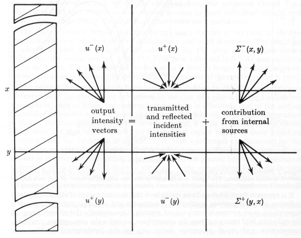
If we consider an arbitrary layer in the atmosphere, bounded by planes with coordinates x and y, a ≤ x < y ≤ b, then the intensities emerging from the layer u+(y), u-(x), depend linearly upon the incident intensities and the sources Σ+(x, y), Σ-(x, y), present within the layer, figure 3. Thus we may write
   u+(y) = t(y, x)u+(x) + r(x,y)u-(y) + Σ+(y, x)
   u-(y) = r(y, x)u+(x) + t(x,y)u-(y) + Σ-(y, x)     (3)
The linear operators t(y,x), t(x,y), r(x,y), r(y,s) present in equation 3 have obvious physical meanings. The first pair are operators for transmission and the second pair are operators for reflection of the radiation field.
The statement embodied within these equations is known as the interaction principle. It is, of course, an exact relationship that contains the entire physics of the problem; valid for all physical situations, namely homogeneous, inhomogeneous, scattering and non-scattering model atmospheres. As we have seen in (4, 5, 6), these equations are themselves a key relationship for analysing radiative transfer problems, for it is possible to relate local physical data and on local physical data through them. Before any analysis may be carried out, it is first necessary to construct the r, t and Σ operators involved in equation 3. This is itself a major problem, particularly if we are concerned with modelling a cloudy planetary atmosphere.
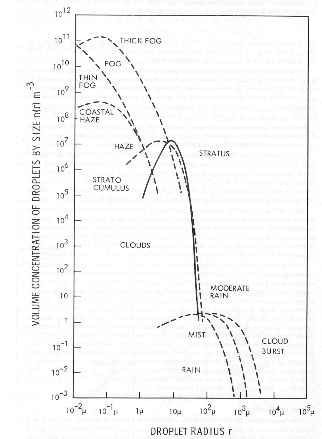
In Figure 4 we have illustrated some typical size distributions of water droplets as they exist in the terrestrial atmosphere in the form of water clouds, rain and fog. These curves may be fitted by a simple mathematical relationship knowing the mode radius and the total number of particles per unit volume, (7). From a knowledge of the drop size distribution it is then a straightforward matter to compute the phase function (or single scattering diagram) for a particular cloud, haze or aerosol, (4, 7).
With all the r, t and Σ operators in equation 3 now constructed for a particular model atmosphere, the theoretical investigator is now in a position to analyse his particular radiative transfer problem. Although in recent years, there has been an avalanche of methods of solution of the transport equation, we do not need them all. A recent critical review of this subject, indicating those efficient and accurate techniques that may be used to analyse problems of the real world, is given in reference 4.
Atmospheric models are classified under two main headings; homogeneous and inhomogeneous and it is important that we know the circumstances in which we may select one and not the other. The choice is wavelength dependent. At wavelengths where there is no absorption by atmospheric gases (window wavelengths), the atmospheric properties depend upon the scattering (cloud) layer and the surface. Consequently at these wavelengths when we are considering continuum effects, a homogeneous model may be used. An inhomogeneous model (physically we mean a gravitational atmosphere) should be used provided that we have accurate information of the vertical variation of the cloud and atmospheric structure. Models of planetary atmospheres must be inhomogeneous at visible, infrared and microwave regions of the spectrum, where we may be computing spectroscopic or thermal features; constructed in such a way that they incorporate the vertical variation of the atmospheric properties (pressure, temperature, relative humidity, clouds...), (8, 9, 10). If this type of model atmosphere is not used for spectroscopic problems, then it will not be possible to reproduce the observed features (9, 10).
In this final section we illustrate some examples of radiative transfer studies that I have undertaken as part of experimental investigations. These examples are just a selection from a large number of investigations that I have made in recent years and they have been chosen to illustrate different aspects of radiative transfer studies.
The Detection of Ice Clouds in the Earth's Atmosphere from a Remote Sounding Experiment: At the present time there is considerable interest in obtaining atmospheric profiles of temperature and composition on a global basis from orbiting satellites.
The most suitable absorption bands for these experiments in the terrestrial atmosphere are the well defined CO2 bands at 4.3 and 15μ since they do not coincide in frequency with any other emissions from various gases present and because CO2 has a constant mixing ratio up to 100 km.
Clouds present themselves as a serious problem to such experiments. Information regarding low clouds may be obtained from high resolution measurements in window channels, but this approach is not effective for high clouds such as cirrus. In order to overcome this problem, Houghton and Hunt (8) have shown that cirrus clouds may be uniquely identified by comparing the thermal radiances at a pair of wavelengths in the far infrared where the absorbing properties of water vapour are the same, but where the properties of ice are considerably different. In addition to observing the presence of cirrus, it has been shown that the thickness of the cloud may be determined from these thermal radiances, even though, in an extreme case, the cloud may not even be visible to the eye. The detailed theoretical studies described in (8) have shown that measurements entered at wavelengths of 50 and 120μ will provide the desired information, and further that supporting measurements near the 2.6μ will provide information regarding the size of the cloud particles. From this extensive study an instrument incorporating these cloud channels into a 15μ. Selective Chopper Radiometer (SCR) has been designed by a team from Oxford/Heriot Watt Universities for remote sensing of the atmosphere that will be flown on the NIMBUS E satellite of the NASA meteorological series, due to be launched in December 1972.
Formation of Absorption Lines in a Cloudy Planetary Atmosphere: The interpretation of spectroscopic data is a fundamental tool for determining the composition and structure of a planetary atmosphere. Clouds again present themselves as a major problem and until very recently no comprehensive theory of line formation in a cloudy atmosphere existed to explain all the observations. The situation was recently rectified by the detailed study described in (9), which was applied to the formation of absorption lines in a Venus atmosphere.
A further development of this work has proved strong evidence for the structure of the visible Venus cloud layers (10). It appears to consist of at least two layers; a dense cloud layer in the troposphere whose top is at a pressure level of about 0.2 atm, with a diffuse haze extending from this level to a pressure of about 5mb in the stratosphere. This additional use of spectroscopic phase curve observations to provide precise information about the structure of the visible clouds, has, hitherto been unnoticed. No other spectroscopic observation or continuum observations such as polarisation measurements can provide this information. It has been shown in (10) that the most suitable observations are those of the weak CO2 bands in the Venus spectrum, such as 7820 and 7883Angstrom. The precise shape of the phase curve (the variation of the equivalent width of a line or band, with phase angle) in the range 0 ≤ i ≤ 120°, provides unique information concerning the structure of the cloud layers. Since the features that we are observing relate to a region of the atmosphere which is in rapid motion, (11), a prerequisite of this type of observation is that the observational time scale is less than the dynamical time scale. This cannot be achieved from Earth. However, spectroscopic phase curve observations of this type are an ideal experiment for an orbiting or fly-by space mission provided that the phase angle range of 0 ≤ i ≤ 120° is observed.
It is apparent from our discussions in this article that we have the tools to provide the theoretical analysis for the majority of radiometric observations. The development of theoretical methods for radiative transfer problems, is an area that has made rapid progress during the last decade and this is certainly associated with the developments of the high speed digital computers. But, theoreticians should be held in check somewhat and not be allowed to run rampant through the physical world ignoring the experimentalists. On the other hand, the experimentalist should not be allowed to stockpile his observations without any detailed theoretical analysis, otherwise it may be impossible to assess the value of his work. The need therefore, is for a compatible marriage between theory and observation.
The future looks extremely promising for planetary meteorology, since with the American and Russian space programs and the ground based observations, it would seem that these projects will provide the type of observations necessary for us to determine and understand the radiative and dynamical properties of the planetary atmospheres in our solar system. Until we have these observations and theories to explain them, we must anticipate difficulties in our understanding of atmospheric systems, It would seem therefore, if we paraphrase Julius Caesar, Act I. Scene 2, that the trouble lies not in our stars but in ourselves.
This paper is published with permission of the Director General of the Meteorological Office.
Part of the work described here was carried out at the Jet Propulsion Laboratory, California Institute of Technology, under contract number NAS 7-100 supported by the National Aeronautics and Space Administration.
1. Goody, R. M. (1964). Atmospheric Radiation, Oxford University Press.
2. Houghton, J. T., and Smith, S. D. (1970). Proc. Roy. Soc., A320, 23.
3. Chandraskhar, S. (1960). Radiative Transfer, Dover.
4. Hunt, G. E. (1971). J.Q.S.R.T., 655.
5. Hunt, G. E. (1972). Rep. Prog. Phys., 26, in press
6. Priesendorfer, R. (1965). Radiative Transfer on Discrete Spaces, Pergamon Press.
7. Deirmendjian, D. (1969). Electromagnetic Scattering on Spherical Polydispersions, Elsevier.
8. Houghton, J. T., and Hunt, G. E. (1971). Q. J. Roy. Met. Soc., 97, 1.
9. Hunt, G. E. (1972). J.Q.S.R.T., 12,387.
10. Hunt, G. E. (1972). J.Q.S.R.T., 12, 405.
11. Goody, R. M. (1969). Ann. Rev. Astron. Astrophys., 7, 303.
