The Classification of a Set of Elements with respect to a Set of Properties

Paul Constantinescu

1966

Paul was a visitor to the Atlas Computer Laboratory in the period 1965-66. He was a major user of the Atlas Algol system with a fiendish delight in using recursion wherever possible.

The paper sets up a formal mathematical scheme to describe the relations amongst a set of elements which may have any of a number of properties in common. The method uses graphs and trees and their matrix representation. The idea of clustering is developed with a note on some problems which have been solved with a general purpose computer program. There is an indication of the possibility of applying the analysis to problems in many different fields.

Let M = (M₁, M₂, . . ., M_m) be a set of elements and P = (P₁, P₂, . . ., M_n) be a set of properties.

One element M_i Î M can have, or cannot have, a property P_k Î P. In order to describe this fact for every doublet M_i and P_k, we shall consider a matrix M₀ with m rows and n columns.

           α11  α12...α1k...α1n
           α21  α22...α2k...α2n
 M0 =      ..................
           ..................
           αm1  αm2...αmk...αmn
         

where the α_ik are 0 or 1 (α_ik ÎL₂):

α_ik = 0 if M_i has not the property P_k

α_ik = 1 if M_i has the property P_k

We consider the linear space of the vectors

α_i = (α_i1, α_i2, ..., α_in)

for which are defined

α_i + α_j = (α_i1+α_j1, α_i2+α_j2, ..., α_in+α_jn)

λα_i = (λα_i1, λα_i2, ..., λα_in)

+ being the sum modulo 2.

In this space we consider the distance

d(α_i,α_j) = p_ij

where p_ij represents the number of unity-components of the vector α_i + α_j, that is the weight of the vector α_i + α_j.

We can describe the distances for all the couples of vectors by means of the matrix M_d of order m:

           p11  p12......p1m
           p21  p22......p2m
 Md =      ................
           ................
           pm1  pm2......pmm
         

This matrix is a symmetrical one (p_ij = p_ji) and p_ij ÎI_n = [0,1,2,...,n] where p_ii=0. We can associate with the matrix M_d one graph G using n+1 levels (level(0),level(1),...,level(n)) as in Figure 1.

Figure 1

For each doublet of elements (M_i, M_j) we draw the branches which go out from M_i and M_j respectively and which meet each other at the level p_ij = d(M_i, M_j), so determining a vertex M_ij on this level (Figure 1).

By drawing, for every doublet (M_i, M_j), the corresponding vertex we obtain the graph G associated with the matrix M_d. We shall call the elements of M initial vertices of the graph G. On this graph we can see on every level the number of doublets of elements of M between which the distance is the number associated with the respective level.

If all the doublets of elements M_i1,...,M_ik are connected by branches on the level (r) we shall consider in the graph G only one vertex M^r _i1i2...ik which is connected by branches with the initial vertices M_i1 , M_i2 ,..., M_ik and which represents all the doublets of elements M_il,..., M_ik (Figure 2).

Definition 1

We say that the level (p) is superior to the level (r) if p ≤ r(p,rÎI_n) (or r is inferior to p). Accordingly, with Definition 1 we shall call the vertices on the most inferior level final vertices.

Figure 2

Definition 2

We shall call a graph G associated with a matrix M_d a tree if it has only one final vertex (on the last level (n) or on a superior one) and if from each vertex (including the initial vertices) only one branch goes out on the inferior levels.

For big m (number of elements of M) we shall use the following representation G' of the graph G: In G' we shall represent only the vertices of G (excluding the branches). Each vertex represents a subset M_i1 , M_i2 ,..., M_ir of elements of M or we can say, all the doublets of elements M_i1 , M_i2 ,..., M_ir .

Definition 3

A representation G' of the graph G is a tree-representation if it has only one final vertex (on the last level (n) or on a superior one) and if on each level it has only vertices M^r _i1...ir for which the sets of indices J_i = (i₁, . . ., i_r) are disjoint.

Definition 4

We shall call absorption of any vertices from the set of vertices M^qj _ij1...ijk , (i_j1 ,...i_jk ) = J_j, by the vertex M^q _i1...il where q = max (q_j) and (i₁...,i_l) = J = U_jJ_j, the transformation of the representation G' into the representation G" in which the vertices M^qj _ij1...ijk , or only a part of these vertices, are replaced by the vertex M^q _i1...il .

Remark 1

Any vertices from the set of vertices M^qj _ij1...ijk can be absorbed by M^q _i1...il (see Definition 4) if, and only if on the levels superior to q there are all the vertices M^qj _ij1...ijk by which all the doublets of elements M_i1 ,..., M_il are represented.

Remark 2

Particularly, by absorption we can get from the vertices - placed on the same level - which represent all the doublets of the elements M_i1 ,..., M_ik , one vertex M_i1...ik (see Figure 2).

Definition 5

A set of initial elements M_i1 ,..., M_il (l < m) which are represented in a tree or a tree representation by M^q _i1i2..il (this vertex may be obtained by absorption) is called a cluster of elements of M. We shall prove the following:

Lemma

A tree-representation tree G' is a representation of the tree G and reciprocally.

Proof

We must prove that if G' is a tree-representation then G is a tree. In fact, if on each level the subsets J_i are disjoint, then from each vertex on the superior levels only one branch is going on this inferior one. The converse is obvious.

Therefore with respect to the trees' or the tree representations' conception the clusters on a given level of the set M are disjoint. The set of the clusters of M represents the classification of the set M with respect the properties-set P.

Since in the general case G (G') is not a tree (tree-representation), in order to obtain a classification of the elements of a set M we need to associate with the graph of the matrix M_d, a tree or tree-representation.

Definition 6

A tree (tree representation) as in Figure 3 is a trivial tree (tree- representation). Let us consider a set of elements M with m elements. We shall prove the following:

Figure 3

Theorem

A representation can be transformed in a non-trivial tree-representation if and only if there are at least two vertices for which the sets of indices J and J' are disjoint where J È J' = 1,2, . . ., m, and from which at least one is not on the last level.

Proof

The condition is sufficient.

A. Let M_J be the vertex which represents the elements having the indices in J; let M_J and M_J' be on the level r and r', respectively (r < r'). Let us consider M_J^* and M_J^** on the level p < r for J^* Ç J^** = k.

(a) If J^* È J^** Ì J then M_J^* and M_J^** can be absorbed by M_J.

(b) If J^* Ì J and {J^** - k} Ì J' then M_J^* and M_J^** can be absorbed by the vertex M_{J È J1}.

Analogously we can reason in the other cases. Therefore, if the condition of the Theorem is fulfilled then on each level we have only vertices according to the Definition 3.

B. We must prove that there is only one final vertex. In fact, if we have - for instance - two final vertices M_αβ and M_γδ for which α,β Î J and γ,δ Î J' then both can be absorbed by M_JÈJ'. We can reason analogously in the other cases of two or more final points.

The condition is necessary.

Actually, if the condition is not fulfilled we can obtain a trivial tree-representation (see Figure 3), or there is at least one vertex from which go out two branches to the vertices on the inferior levels.

The binary case we considered so far is not material; all these considerations are valid if the elements of the matrix M₀ are integers. Any suitable distances can be chosen too.

Example. Let

           --                      --
           |  1  0  1  0  1  1  1   |
           |  1  1  0  1  1  1  0   |
           |  0  1  0  1  1  0  0   |
      M0 = |  1  0  1  0  0  1  1   |
           |  0  1  1  1  1  1  0   |
           |  1  1  1  1  1  0  0   |
           |  0  0  1  0  0  1  1   |
           |  0  1  1  0  1  1  1   |
           __                      --

The matrix M_d is:

           --                         --
           |  0  4  6  1  4  4  2  2   |
           |  4  0  2  5  2  2  6  4   |
           |  6  2  0  7  2  2  6  4   |
      M0 = |  1  5  7  0  5  5  1  3   |
           |  4  2  2  5  0  2  4  2   |
           |  4  2  2  5  2  0  6  4   |
           |  2  6  6  1  4  6  0  2   |
           |  2  4  4  3  2  4  2  0   |
           __                         --

The representation G' is the following:

Level
(1)       M14       M47
(2)  M23       M25  M35  M36  M26  M56  M17  M18  M58  M78
(3)                      M48
(4)            M12  M15  M16  M38  M57  M28  M68
(5)                      M24  M45  M46
(6)                 M13  M37  M67  M27
(7)                           M34

By absorptions we obtain, e.g. the tree from Figure 4.

Figure 4

The algorithm which we can deduce from the above considerations, in order to solve a given problem of classification of a set M in respect to a set of properties P needs the following steps:

1. The calculation of the matrix M_d and of the graph G from the given matrix M₀

In any of the ALGOL programs for clustering (Atlas Laboratory, Chilton, Didcot, Berks., or Computing Center, University of Bucharest, Rumania) we describe the graph G by two arrays G1[i,j] and G2[i,j] where i represents the levels (i = 1,..., n) and j represents the first (in G1) respectively, the second (in G2) vertex of every couple on the level i..

For instance, in the example considered above we have

G1: 14                        G2: 47 
    1122233557                    7835656688 
    4                             8 
    1112356                       2568878 
    244                           456 
    1236                          3777 
    3                             4

2. The calculation of the trees associated with the graph G

In order to obtain all the trees (tree-representations) which are associated with the graph G we shall describe on every level all the subsets of M which fulfill the following conditions:

1. The subsets are obtained by absorptions (procedure TRIANG, Figure 5).
2. On every level we write those subsets which are not included in the subsets on the superior levels (including the preceding subsets on the level in discussion), (procedure INCLUD, Figure 5).

According to the definition of the absorption, in order to get a vertex M_i1...ik i.e. a subset (i₁...i_k) on the level j, we must verify that on the levels superior to the levels j (including j) there are all the couples (i₁,i₂), i₁,i₃),...,i₁,i_k), i₂,i₃),...i₂,i_k),... i_k-1,i_k),

For this purpose we consider the arrays T1[i] and T2[i,j]. In T1, i describes the index for all the couples (having i as first index) which are on the first b levels in G1 and G2; in T2 j describes the corresponding indices from G2.

For instance, in the example mentioned, if b = 4 we have:

T1: 1          T2:245678
    2             3568
    4             78
    5             678
    6             8
    7             8

In order to fulfill the condition (a) we can remark that the absorption takes place if and only if all the elements on each parallel to the first diagonal in T2 are equal (procedure TRIANG).

It can be illustrated if we consider for instance the couples (1,2), (1,3), (1,4), (1,5), (2,3), (2,4), (2,5), (3,4), (3,5), (4,5) and the corresponding arrays T1 and T2:

T1: 1          T2:2 3 4 5
    2             3 4 5
    3             4 5
    4             5

In order to fulfil the condition (b) we verify that every subset which satisfies the condition (a) is not included in a preceding one. Finally, we get a pattern which contains all the trees we can associate with the graph G (the subsets on the level b are called R(b,i,j) in Figure 5).

In the example considered above we get the following pattern:

Level  (1)   (14), (47)
       (2)   (147), (178), (2356), (58)
       (3)   (1478)
       (4)   (12568),(23568),(578)
       (5)   (124568),(14578)
       (6)   (1235678),(145678),1245678)
       (7)   (123456768)

The tree considered as an example above (Figure 4) is shown up by the tree-representation which produces the underlined clusters. We notice, for instance, that (12345678) = (1478) È (2356) satisfies the condition of the Theorem.

According to the Theorem given above and other supplementary considerations connected with the physical character of the problem (technology, economy, biology, etc.) we can select from the final pattern the particular tree-representations which produces the clusters in M.

Since such problems of classification of the information appear in many fields, this way of producing the final pattern seems to the author to be suitable in order to be able both to solve a large class of problems and to create the possibility of interfering with the supplementary conditions required by each particular problem.

Certainly such supplementary conditions can be formulated even for the algorithm which, with the corresponding modifications, can lead, for instance to, instead of the pattern, only one tree-representation.

As a result of such conditions, five variants of the basic algorithm described above were written:

Cluster 1.

Produces almost all the subsets providing almost all the clusters (trees). Recommended in the range m < 30. We must note that for instance in the case of m = 30 we can get about 200 subsets on one level in the final pattern.

In order to reduce the number of subsets but to maintain, as much as possible, the same number of trees furnished by the final pattern, the following three variants can be used:

Cluster 2.

Produces on each level at the most m subsets (for each possible initial element in each subset, at the most 1 subset). Recommended in the range m < 50. The decreasing of the number of trees furnished by the final pattern is much smaller than the decreasing of the number of subsets.

Cluster 3.

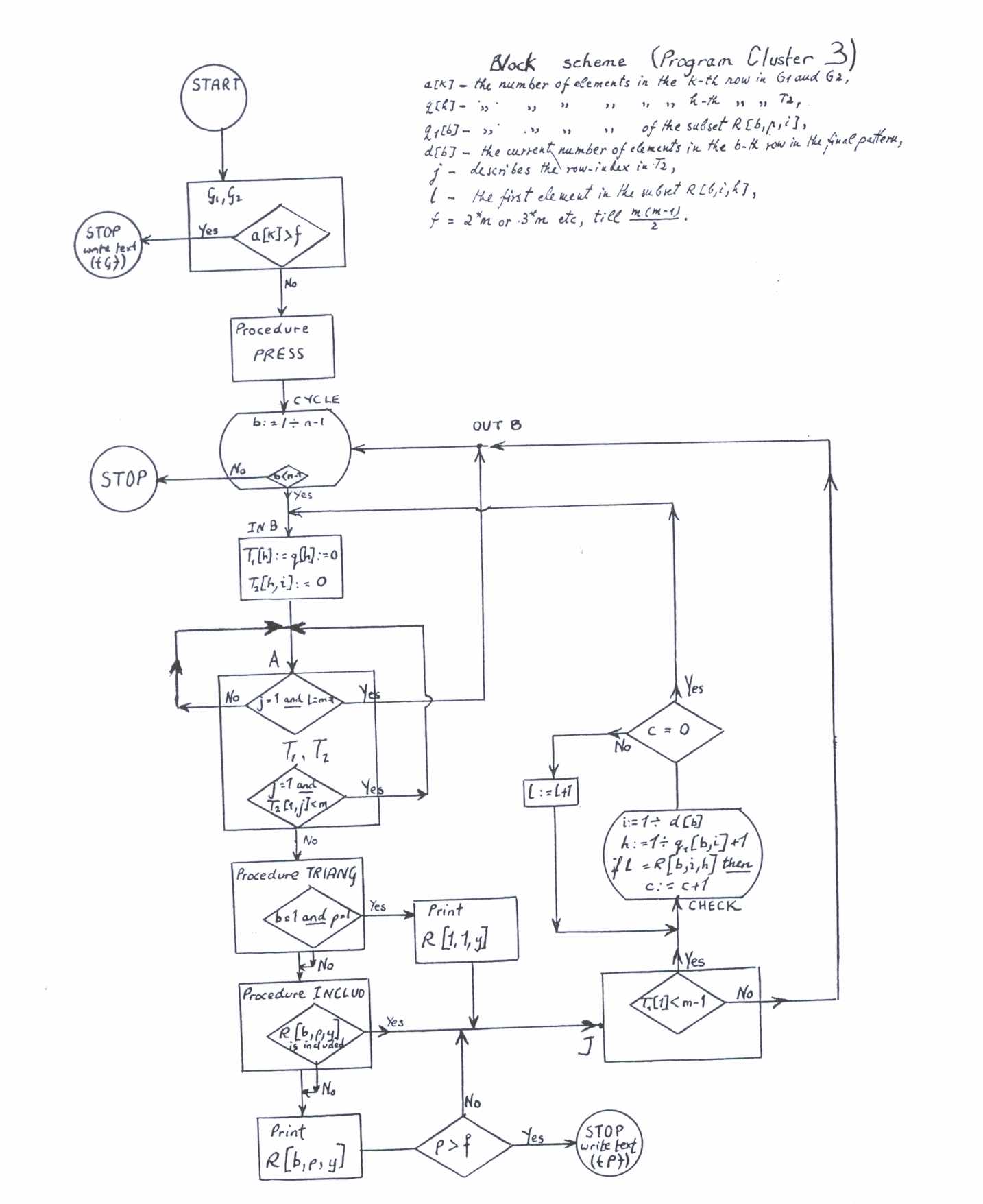
From the subsets which can be produced by Cluster 2, it keeps on each level only the subsets which are partial disjoint (every initial element is not in the precedent subsets on the respective level). Recommended in range m < 50. The block scheme in the case of Cluster 3 is given in Figure 5.

Cluster 4.

The subsets in the final pattern arc on every level almost disjoint (excluding the last element in every subset, the subsets on a given level are disjoint). Recommended in the range m < 100.

In order to get a satisfactory number of trees from the final pattern, the number of required levels is in general much smaller than n. In fact, if, for instance, n = 100, then for about 10 levels (recommendably in the range between levels 40 and 50) we can get a pattern furnishing enough trees which would satisfy the most exacting researcher.

Clusters 1, 2, 3, 4 were used for different problems from Psychology, Biology, Electrical Designing, etc. In the ranges mentioned above, every problem could be solved at the most in 15 minutes on Atlas. For instance, a problem with m = 30 and n = 70 is solved by Cluster 3 in 2 minutes if we ask for the pattern with about 20 levels, which provides enough information in order to get a rich set of trees. For m = 50, Cluster 4 gives about 20 levels in 4 minutes.

In order to deal with bigger amounts of data (m < 1000) another variant has been provided:

Cluster 5.

Produces subsets only on a certain level in every case of Cluster 1, 2, 3, or 4. We can get some nodes of the trees containing the clusters if we apply Cluster 5 for certain levels. In this way we can use even Cluster 1 for a bigger m if we are interested in overlapping subsets on a given level.

For every variant, ALGOL programs depending on the initial data were elaborated: for integral or binary numbers, in both cases. when all the elements of the matrix M₀ are known or not. In the case of incomplete data some solutions are considered in Constantinescu and Stringer. The preparation of the matrices of distances M_d in the sense considered by Bonner (1964) is recommended in the case of Clusters 3, 4.

A more complete description of the algorithm, illustrated in the cases of Cluster 1 and Cluster 4, is given in Constantinescu.

Conclusions

1. It appears that the definition of Cluster introduced in this paper fits a larger class of problems than the previous concepts. Moreover, it contains that known by the author as a particular case: for instance, the clusters conceived by Bonner (1964) as "maximal complete subgraphs of the similarity matrix graph" can be obtained from Definition 5 when considering only the elements which are at distance 1 (level 1).
2. This point of view for clustering leads to an algorithm which seems to be versatile enough even if we take into account only the five variants operating in the range 1 < m < 1000. But further variants might be available.
3. Generally speaking, the Cluster Analysis of the type described above, and Factor Analysis can be considered complementary. It stems especially from the fact that, in the case of Cluster Analysis, the number of properties (n) practically does not affect the computing time, and therefore Cluster Analysis can be used for the problems with which Factor Analysis does not deal easily; and conversely. A more detailed discussion concerning this comparison is developed in Constantinescu and Stringer.
4. A way which might blend some advantages from both Cluster and Factor Analysis seems to be that indicated in Howard (1964). But although conditions for keeping the configuration of the points within a sphere, during suitable transformations (for instance, projecting successively the initial configuration in consecutive subspaces), are increasingly available, the problem of rejecting artificial similarities, produced by these transformations, seems to lead to conditions too stringent to be effective. Nevertheless, at least for some classes of problems, such conditions might be conceived.
5. The rich list of applications, "mechanical translations, psychology, information retrieval, artificial intelligence. semantics, determination of species, scientific classification, general systems, architectural planning, philosophy and the theory of art generally," given in (1) could, however, be extended.

For instance, we can add certain more technical applications such as: the synthesis of computers or more generally the synthesis of finite automata (the coverings of a graph with a set of subgraphs as a step in the synthesis), classification of patents, classification of different technical procedures, problems of prognosis in meteorology, economical planning, theory of codes, etc.

I should like to express my gratitude to Mr. Alex Bell (Atlas Laboratory, S.R.C.) for his constructive remarks concerning the programs in Atlas ALGOL.

My debt to Dr. J. Howlett and Dr. R. Churchhouse (Atlas Laboratory, S.R.C.) for their help in all spheres of my work at the Laboratory is considerable and I owe them much for their assistance.

References

GOOD, I. J. (1962). The Scientist Speculates: An Anthology of Partly Baked Ideas. Heinemann, London; Basic Books, New York.

BONNER. R. E. (1964). "On Some Clustering Techniques," IBM Journal, January, 1964.

HOWARD, R. N. (1964). "Classifying a Population into Homogenous Groups," Proc. of International Conference of Operational Research Society - Cambridge 1964 (forthcoming).

CONSTANTINESCU, P., and STRINGER, P. "On the Cluster Analysis of Incomplete Matrices in Personal Construct Theory" (sent for publication to Psychometrika).

CONSTANTINESCU, P. "On Cluster Analysis" (Brit. Journal for Statistical Psychology - forthcoming).