
The nuclear three-body problem has for a long time been a source of fascination and frustration to theoretical physicists. If we observe the way in which two elementary nuclear particles (nucleons) interact in isolation we find that their motion can be quite well described, over a large energy range, in terms of an assumed conservative force acting between them. If we allow three nucleons to interact simultaneously there will, presumably, be three such forces acting, one for each pair of particles. If we assume these forces to be the only source of interaction between the three particles, we can write down the equation of motion for the three-body system, and ask whether its solutions agree with experiment as well as do the corresponding two-body equations. Unfortunately, these equations of motion lead to six dimensional coupled partial differential equations, and these cannot be solved directly with currently available techniques and computers.
We can reduce the equations to more manageable proportions by studying only a limited range of three-body problems. Two nucleons form a single bound state, the deuteron, while three nucleons can also form a three-body bound state, the triton. The simplest three body problems are those describing the triton, and the elastic scattering of the third nucleon from a deuteron. The equations describing these situations reduce, when we take account of the rotational symmetries, to a finite set of coupled three-dimensional partial differential equations.
Whether we can solve these equations directly depends on what assumptions we make about the forces between two particles. With the simplest assumptions, we get only one equation, and with current techniques it is just possible to solve a single partial differential equation in three dimensions by finite difference methods. But these assumptions are not valid in practice; with the type of force which fits the two-body experiments, we get, not one but (in the simplest case) sixteen coupled partial differential equations. It is these sixteen coupled equations which we are trying to solve on Atlas.
The difficulty of solving M coupled partial differential equations is approximately proportional to M3 and a direct finite difference solution is not very practicable. Instead, we use a variational method (or rather, a variety of variational methods). These involve expanding the solution in a series of known functions, and determining from the equations of motion the unknown expansion coefficients; the original set of partial differential equations is thus replaced by an algebraic set of (linear) equations for these coefficients, which can be solved trivially. The work involved lies wholly in setting up the equations. If we keep N terms in the expansion of the solution, we obtain a set of (roughly) 16 N linear equations for the 16 N unknowns (remember, we have 16 coupled equations !). Each term in these equations involves an integration of a rather messy function over the three dimensions in which the equations are defined; the time is spent in doing these three dimensional integrals to the necessary accuracy.
The numerical integrals which have to be performed are of the general type
Iij = ∫ fiHijfj dτ
where fi (x), fj (x) are M-vectors defined over a three-dimensional space x, and Hij(x) is an M × M matrix of differential operators in the space. The form of H, and the value of M, depend on the particular three-body state considered, and in particular on the total angular momentum of the system. For the simplest angular momentum state (J = ½ in the units used) M takes the value 16 quoted above. We approximate Iij by a numerical integration over a discrete set of points at which we must evaluate the appropriate integrals and the form of the programme is determined by the two difficulties which arise. These are :-
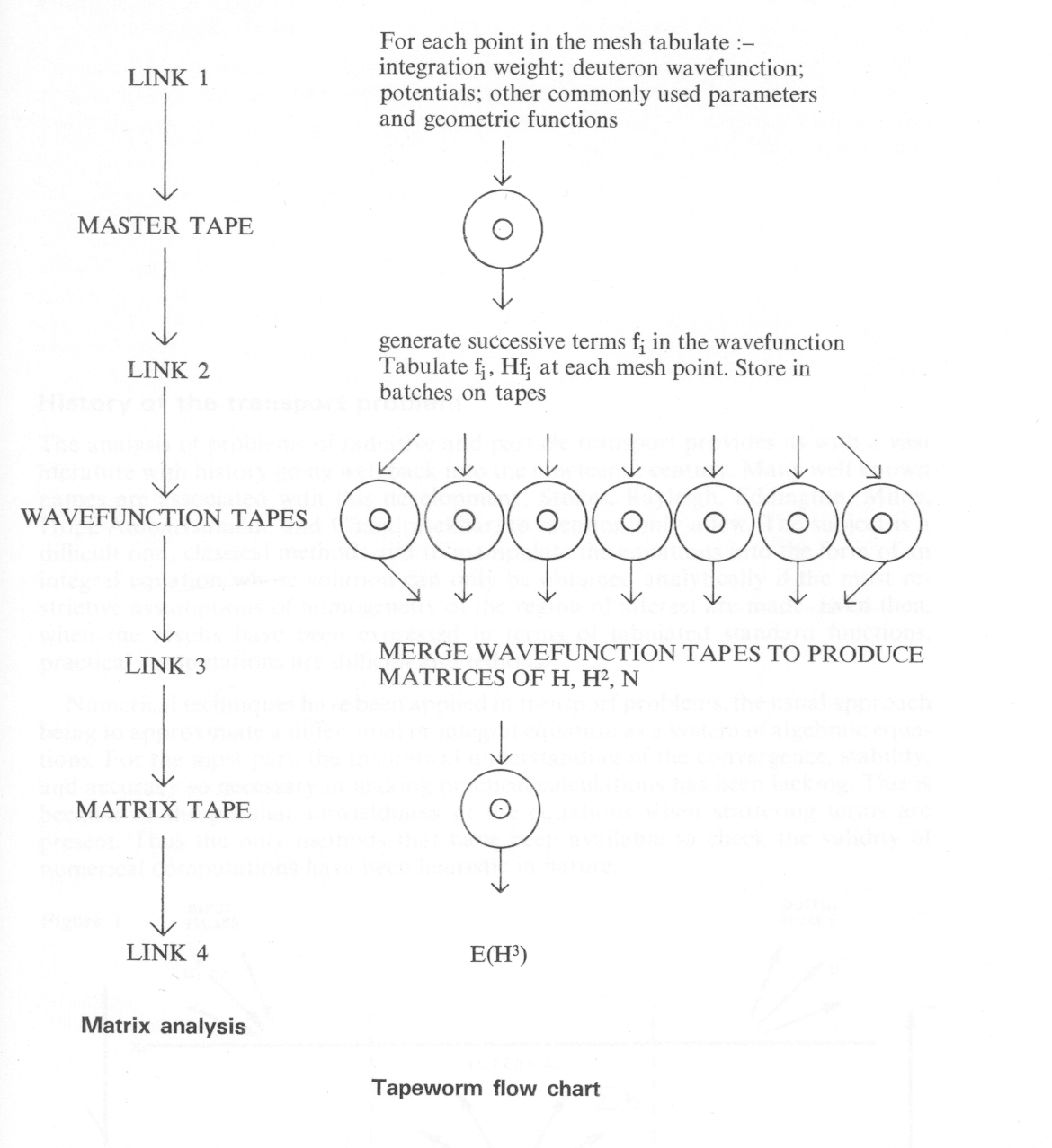
We have alleviated the first difficulty by providing a set of subroutines for manipulating automatically the three-dimensional functions together with their first and second derivatives. Even so, the checking required to guarantee the relevant coding has reached several man years. We have also coded fully automatically the operator matrices Hij, so that the programme is not limited to a particular value of the angular momentum. The second difficulty we remove altogether by writing to tape the functions fi (x). HFi (x) for each x in the numerical integration mesh, and for each i =1,N. The integrals Iij are then produced later in a final grand merging run. This final run is relatively fast, and hence in this way the time taken has a leading term proportional only to N. Since N becomes quite large in practice (of order 40) we accumulate tapes rather rapidly, together with the associated problems of editing and maintenance. The rate at which the programme eats tapes led to its descriptive name; a simplified flow diagram of the complete programme is shown in Fig. 1.
The programme produces as its final output upper and lower bounds on the triton binding energy. and variational approximations to a number of parameters that characterize nucleon-deuteron elastic scattering. A considerable amount of running has been done so far, and the results are encouraging; the current series of runs is designed to improve the bounds already obtained, and to provide checks on the numerical accuracy of the calculation.
This work has spread over several years and is continuing. In this time I have had good reason to be grateful to a large number of members of the Atlas Computing Laboratory staff. The programme is written in Fortran, with the exception of the dump and restart procedures. I am grateful to Paul Bryant for providing these facilities, and to E. B. Fossey and Barbara Stokoe for their aid in converting the programme to run under Hartran (starting at a time, in late 1964, when both TAPEWORM and Hartran were rather unsteady infants anyway). Finally, I am very grateful to Dr.J. Howlett for providing the facilities and hospitality of his laboratory, and for the machine time used.
