Time Series Analysis on Atlas - BOMM

Peter Kent

1966

Observations on a system which changes with time form what is known as a time series. Although always referred to as a time series, the same analysis can be performed on series that vary with distance or any similar parameter. As examples of time series we may consider the records of atmospheric temperature or pressure at a particular place, the gold and dollar reserves in the UK, or the depth of the ocean measured at regular intervals across the Atlantic.

Many such series have dominant frequencies of oscillation. Air temperature records for example vary with the seasons and with the time of day. However in addition to these regular fluctuations there are slow changes from year to year and high frequency changes from day to day or even hour to hour. Time series analysis is a method of examining the structure of such series.

A system of programs for performing this analysis BOMM [1] is now working on Atlas. BOMM enables data to be accepted in a wide variety of formats and manipulated according to a sequence of control statements. These control statements allow one to define a variety of input and output forms, to truncate, sort, join, merge, interpolate or plot series, and also to perform various transformations on the series such as taking logs, cross correlations, convolution, or Fourier transforms. There are also statements that allow one to generate series for use as digital filters or lag-windows.

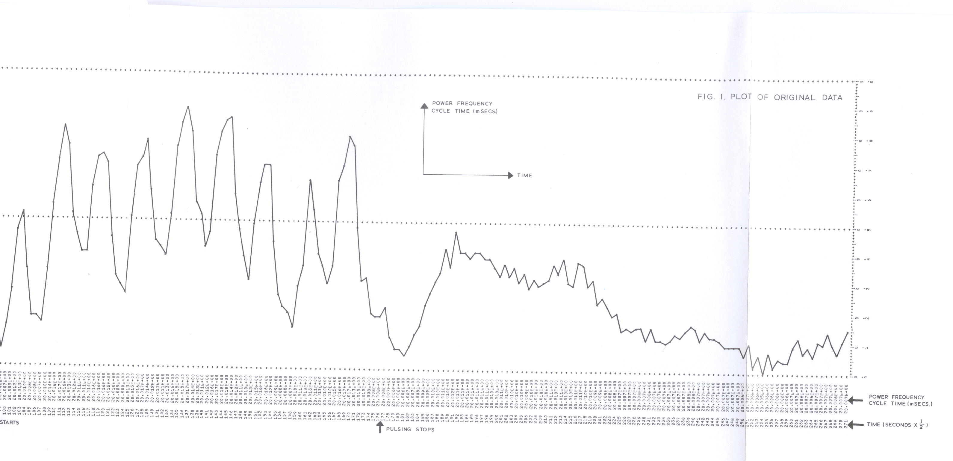
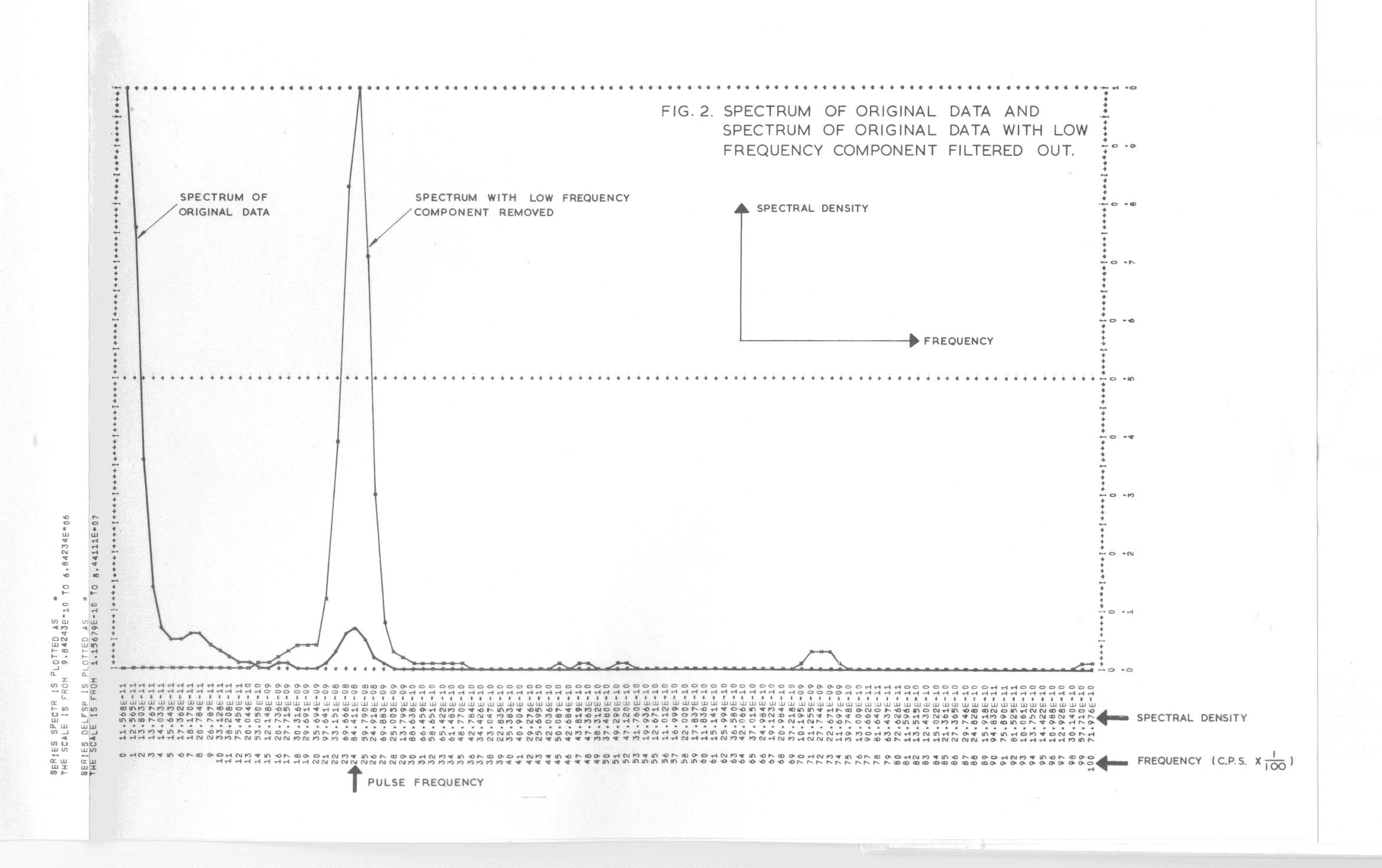
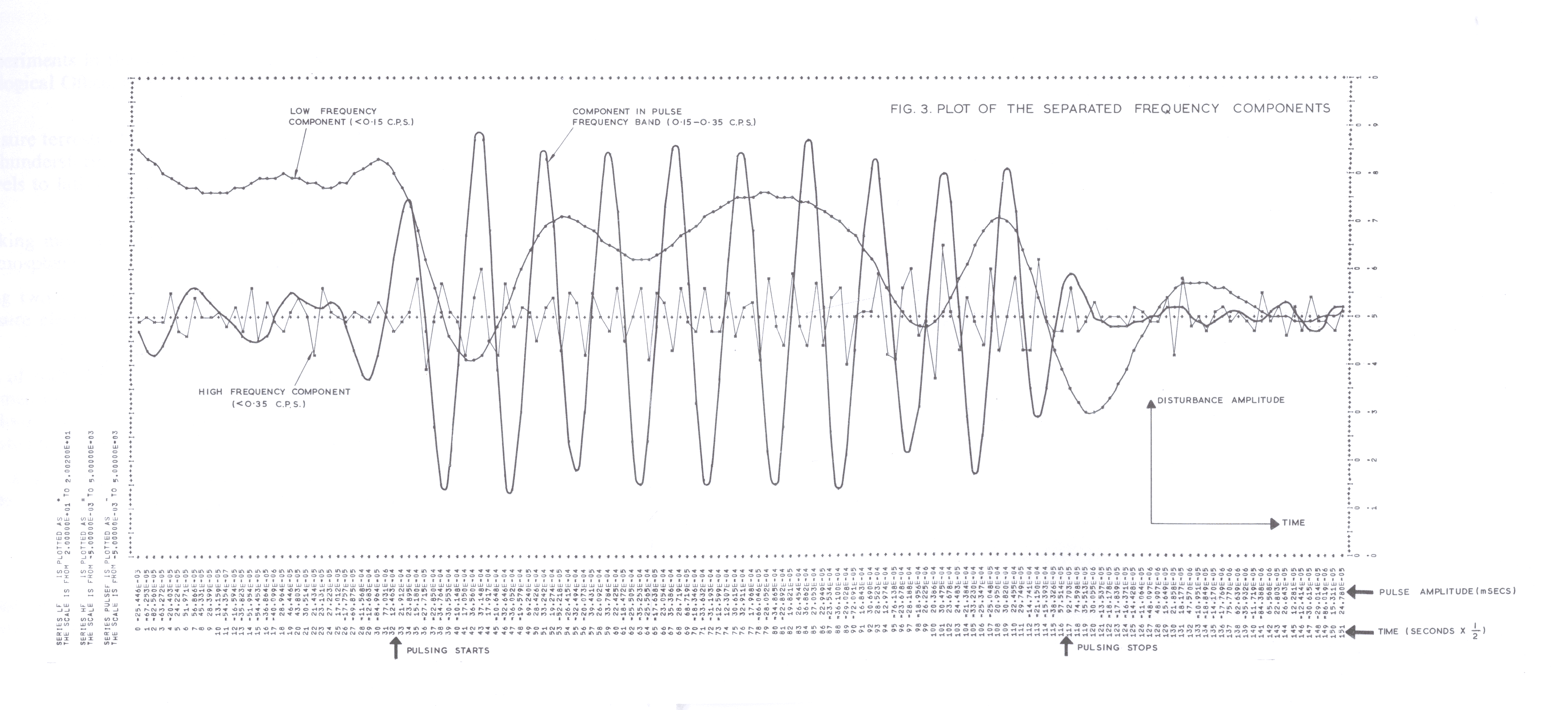
A good example of the use of BOMM was provided by a study undertaken by the SRC and the CEGB [2,3] to determine the behaviour of large interconnected transmission/generation systems when subjected to heavy pulsed loads. The pulses were produced by repetitively exporting electricity to France via the cross-channel link at Lydd. In this way a train of 15 to 25 square waves was produced having amplitudes of 80 or 160 MW and repetition rates of 0.25, 0.33 and 0.5 cycles/sec. The effect was measured at three places in the UK and also at CERN in Switzerland. This was done by timing ten successive 50 c/sec power cycles by means of a 10 Mega-cycle crystal controlled oscillator. The results were printed out at ½ second intervals with an accuracy better than 0.01%. The analysis of this series proceeded as follows :-

1. The original series was read in and then plotted using the data sampling rate as the reference time base. This is shown in Figure 1. The ordinates are automatically adjusted to the maximum and minimum values of the series unless otherwise defined.
2. A spectrum of the series was computed by forming the autocorrelation function, multiplying by a lag-window and then computing the cosine transform of the result.
3. The low frequency component of the series was removed by convolution with a numerical filter and a new spectrum computed. Both spectra were then plotted. See Figure 2.
4. In order to isolate the pulse we consider the original time series S to consist of three components :- high frequency H, pulse frequency P and low frequency L. i.e. S = H + P + L. The first filter applied to S removed L to produce a series H + P. A second filter applied to S removed H to produce a series L+ P. By subtraction of these series, term by term, the three components H, P and L were obtained and plotted. See Figure 3.

The whole analysis was defined by 21 BOMM control cards and took about 30 seconds of computing time on Atlas.

References

1. Bullard, E. C., Oglebay, F. E., Munk, W. H. and Miller, G. R. 'A user's guide to BOMM. A system of programs for the analysis of time series', 1966. The Institute of Geophysics and Planetary Sciences, La Jolla, California, U.S.A.

2. Fox, J. A., Kent, P. 'Frequency variation of United Kingdom Electricity Grid System during the 90 MV A cyclic pulse loading tests on 14/15th November 1967'. Rutherford Laboratory, Chilton, Didcot, Berkshire. 31st December 1967. E/PS-DS/300 GeVJAF-3.

3. Fox, J. A., Kent, P. 'Cross-channel pulse power tests between U.K. and France - 20/21st June 1968. Analysis of power system frequency disturbance.' Rutherford Laboratory, Chilton, Didcot, Berkshire. 1st August 1968. E/PS-DS/300 GeV/JAF-4.