
Numerically computed forecasts of pressure patterns on the scale of anticyclones and large depressions are being produced operationally by several national meteorological services, including the British Meteorological Office, for periods of up to three or more days ahead and these forecasts are claimed to be superior to those produced by more conventional methods. Unfortunately such computer produced forecasts do not and are not able to deal with the problem of forecasting rain quantitatively. Relatively simple models of the atmosphere are used to produce these forecast pressure patterns: the horizontal grid is spaced at intervals of about 300 km and time steps of about 30 minutes are used in the integration. The horizontal dimensions of the large pressure systems are of the order of several hundreds of kilometres and the grid resolution is adequate therefore for handling these systems. It happens however that the features which produce rain have much smaller horizontal dimensions than this and some of the assumptions made in producing forecasts on the scale of the large pressure systems are no longer so valid when' applied to smaller scales of motion. Among these smaller rain-producing features, the organized rain areas associated with the frontal zones separating air masses of different origin are very important features. In order to study the dynamics of fronts and, if possible, to predict the rainfall at these fronts, the British Meteorological Office has carried out experiments in recent years with a more sophisticated model of the atmosphere, using a finer grid and a shorter time step [1,2,3]. The atmosphere as represented in this model is still basically a fairly simple one: despite this, and even though the whole of the SRC ATLAS computer is used on a non time-sharing basis, it takes nine hours of real time to carry out the integrations to produce a twenty-four hour forecast. During this time the computer carries out something like 7 x 10⁹ machine instructions.* ABL (machine code) language is used.
* This is a mean rate of about 220,000 instructions a second. which is much lower than the normal rate of about 350.000. The reason is that the program requires much more main store than is available in the 48 K core store. so that much time is taken up in drum transfers. J. Howlett
The pressure exerted at the earth's surface by the atmosphere is about 1000 mb: pressure decreases with height falling to 500 mb at about 5½ km and to 100 mb at about 16 km. Pressure, p, is used as the vertical co-ordinate in the 10-level model: the heights, h, of the ten pressure levels at 100 mb intervals from 1000 mb to 100 mb define the structure of the atmosphere. The horizontal co-ordinates x, y are taken on a stereographic projection. Horizontal components of wind dx/dt, dy/dt (written u, v) are used to define the horizontal flow at each of the ten pressure levels. Humidity mixing ratio, r, was chosen as the moisture parameter: the particular values used are the mean values of r appropriate to the 100 mb layers centred about 950, 850. . . 350 mb and the atmosphere is assumed to be dry above 300 mb. The above four quantities h, u, v, r, constitute the dependent variables. The vertical component of velocity dp/dt (written ω), is obtained when required via the continuity equation as indicated in the next section. No ice stage is represented in the precipitation process in the model. Additional assumptions about the atmosphere are that it is hydrostatic and inviscid and, in the first experiments, the effects of friction and topography were ignored.
The thickness, h', of the 100 mb slabs between adjacent levels of the atmospheric column above a grid point is a measure of the mean temperature of the appropriate 100 mb thick slab in the atmosphere above that grid point and the thermodynamic equation is expressed in terms of layer thickness, h'. In order to deal with condensation and evaporation effects it is necessary to determine whether or not the air is saturated and such determination is made by comparing the humidity mixing ratio of a particular 100 mb thick slab with the value of the humidity mixing ratio which would be required to saturate that particular slab. Fortunately the saturated humidity mixing ratio, rs, can be expressed as a quartic polynomial in h' to a high degree of accuracy. Naturally, different polynomial coefficients are required for each of the seven layers for which it is necessary to determine rs, but even so only a relatively small number of coefficients need therefore be stored in order to carry out this comparison. Transfer of liquid water from one layer to the layer below can only take place when the slab is saturated at the beginning of a time step and when the rate at which water is arriving both by advection and as liquid water from above is greater than that required to keep the slab saturated. allowing for changes in the temperature of the slab. The latent heat due to evaporation and condensation is included in the thermodynamic equation.
(a) The horizontal equations of motion are used in the form
where m is the map magnification factor sec2(π/4 - θ/2), θ being the latitude, ω is equivalent to dp/dt and f is the Coriolis parameter.
(b) The equation of continuity is expressed in the form
The vertical velocity at each level is obtained by integrating this equation with respect to p by using the trapezium rule. The boundary condition at 100 mb is taken as ω100 = 50 (∂ω/∂p)100 which is consistent with ω = 0 and ∂ω/∂p = 0 at p = 0.
(c) The hydrological equations
If MA is defined as the rate of transfer of liquid water into a layer from the layer immediately above and MB as the rate of transfer of liquid water into the layer below then M, the rate of condensation in the layer is defined by M = MB - MA and M will be negative for evaporation. MA = 0 for the layer between 300 and 400 mb since the atmosphere is assumed to be dry above 300 mb. After testing whether the slab is saturated. the integrations follow whichever is the appropriate of the following alternatives.
If r < rs, ∂r/∂t is given by
and MB = 0. If
and MB = (∂r/∂t)DRY - (∂rs/∂t) unless the value of MB thus computed is negative when ∂r/∂t = (∂r/∂t)DRY and MB = O.
(d) The thermodynamic equation is written as
where L is the coefficient of latent heat of condensation, γ is the ratio of the specific heats and are the arithmetic mean values of u, v, ω at the pressure levels at the top and bottom of the layer whose thickness is h'.
(e) Height tendency equation
Assuming W ≡ dz/dt = 0 at 1000 mb, the tendency equation can be written as
using a one-sided difference to determine ∂h/∂p:ω, u, v, ∂h/∂x and ∂h/∂y
apply to the 1000 mb level and h' is the thickness of the 1000--900 mb layer.
The essential feature of the finite difference scheme used [4] is that it is staggered in both time and space. The complete grid consists of 95 x 63 points approximately 50 km apart and there are 10 levels in the vertical. If the grid points are represented by integers (i,j), i ranging from 0 to 94 and j from 0 to 62 then at even time steps the dependent variables are kept as follows:
  h at i even, j even
  u at i even, j odd
  v at i odd,  j even
  r at i even, j even and ω is computed for i odd, j odd.
At odd time steps
  h is kept at i odd,  j odd
  u is kept at i odd,  j even
  v is kept at i even, j odd
  r is kept at i odd,  j odd and ω is computed at i even, j even.
As the geographical area for which the initial data are taken varies from one case to another so the maximum step, δt, permitted by computational stability criteria also varies. The determining factor is the grid length appropriate to the most southerly latitude of the computation area. So far the time steps used have ranged from 90 seconds to 108 seconds.
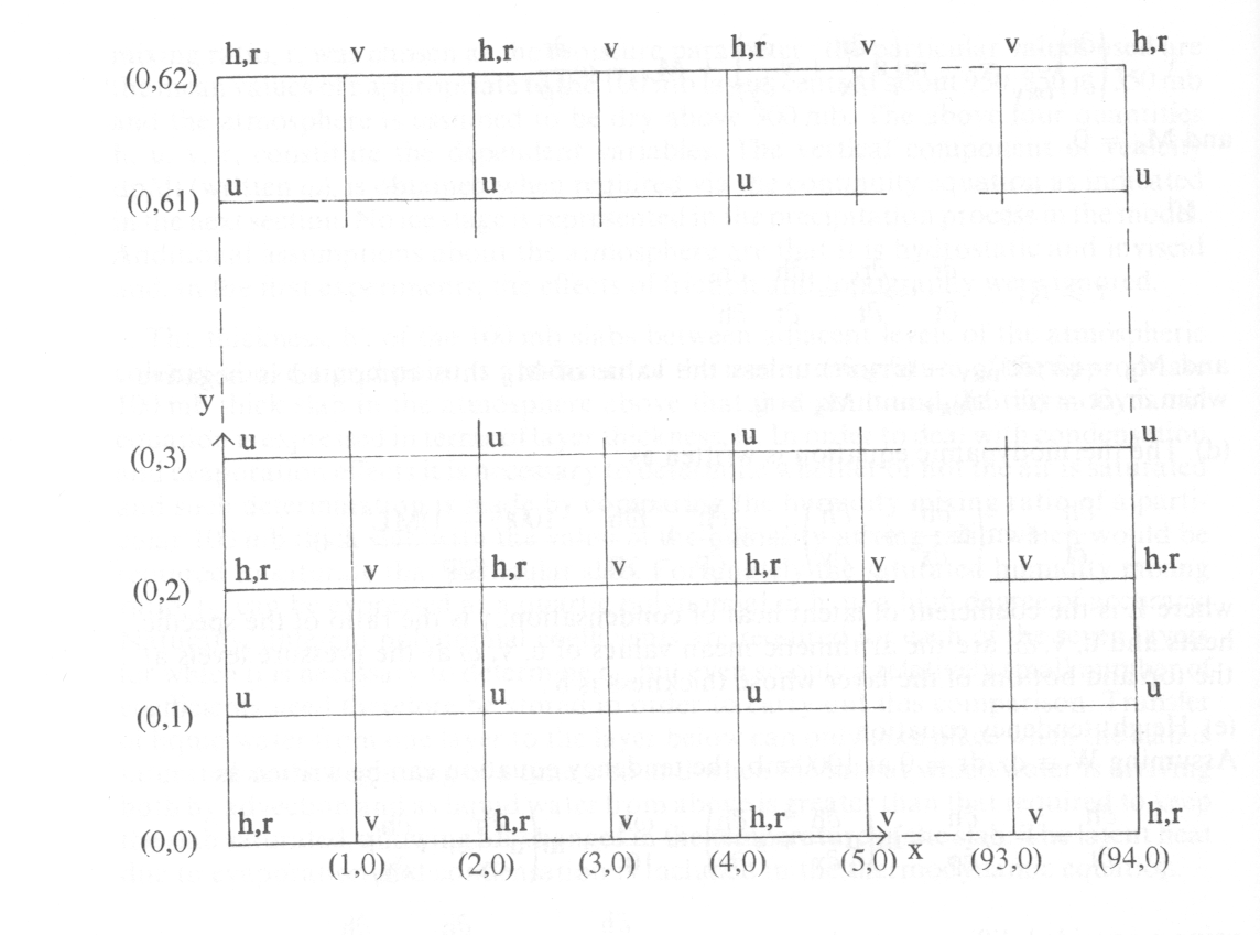
Grid Points (i,j) on 95 × 63 grid with the dependent variables shown as used at even time steps.
Simple three point centred differences are used for the space derivatives except at the boundaries where one-sided differences are normally used. For the vertical derivatives at the top boundary of the model (100 mb) a one-sided difference is a poor approximation and instead a constant determined from the ICAN standard atmosphere is used, corrected however to allow for the appropriate atmosphere at that level as represented in the model. When, in the non-linear terms a variable or its derivative is required at a grid point at which it is not available, a simple average is taken of the values at neighbouring grid points at which the quantity has been computed. Such a scheme introduces sufficient smoothing to ensure computational stability [5] but computational instability can arise if a simple centred difference formula is used for the time derivatives since the nature of the equations is such that two distinct computational modes are set up, one for odd and one for even time steps. The following system of integrating with respect to time has been adopted for all variables
In the early stages of the project one of the biggest difficulties was the control of spuriously large accelerations and divergences near the lateral boundaries: this has been solved by introducing an appropriate diffusion term kV2u, etc., into the equations of motion and the thermodynamic equations, using a physically realistic value for k over most of the field but a larger order of magnitude for k around the outer three rows of the grid.
A record is kept throughout the computations of the accumulated rain falling at grid points i even, j even (excluding the outer boundary grid points): instantaneous rates of rainfall are computed at grid points i odd, j odd at specified even time steps for comparison with the present weather plotted on actual weather charts for the corresponding times.
It was decided that a suitable initial state was to assume that the wind fields be non-divergent: these wind fields are computed from vertically and horizontally smoothed initial height fields by solving the equations
at each level. A suitable boundary condition for the stream function equation is to assume the normal component of velocity to be as nearly geostrophic as possible. A simpler stream function equation, viz. was used in the earlier experiments [l] but the inclusion of the additional term virtually removed a small amplitude inertio-gravitational wave oscillation which had been observed in the forecast fields obtained from the first experiment [3].
Real initial data were used in all the experiments and it is perhaps of interest to comment that the forecast rainfall patterns obtained from this 10-level model are very encouraging and bear close resemblance to the rainfall patterns which actually developed. More recent experiments include the effects of friction and topography as well as convective adjustments to allow for sub grid scale motions which cannot otherwise be represented in the model.
This paper is published by permission of the Director General of the Meteorological Office.
1. Bushby, F. H. and Timpson. Margaret S. 1967. A 10-level atmospheric model and frontal rain. Quart. J. R. met. Soc., London, 93, 1-17.
2. Benwell, G. R. R. and Timpson. Margaret S. 1968. Further work with the Bushby-Timpson 10-level model. Quart. J. R. met. Soc., London, 94, 12-24.
3. Benwell, G. R. R. and Bretherton, F. P. 1968. A pressure oscillation in a IO--Ievel atmospheric model, Quart. J. R. met. Soc., London, 94, 123-131.
4. Eliassen, A. 1956. A procedure for numerical integration of the primitive equations of the two parameter model of the atmosphere. Sci. rep. 4. Contract AF 19(604}-1286.
5. Phillips, N. A. 1962. Numerical integration of the hydrostatic system of equations with a modified version of the Eliassen finite differences grid, Proc. Int. Symp. Num. Weath. Pred., Tokyo, Nov. 7-13, 1960, pp. 109-119.
