
The most powerful computer in Europe. together with an advanced numerical model of the atmosphere. will soon be used for direct forecast of rainfall. Forecasts will be produced within 30 minutes of atmospheric data being available. and will discriminate between steady rain and showers.
Dr Alan John Gadd is scientific officer in the Meteorological Office, Bracknell. He has worked on the incorporation of the effects of surface heating and cumulus convection into the Meteorological Office's 10 level numerical weather prediction model. and he is currently doing further work on this model.
LATE NEXT YEAR the Meteorological Office at Bracknell is to take delivery of what will then be the most powerful computer In Europe. Using this machine it will be possible to adopt far superior methods of weather prediction, providing for the first time direct computer forecasts of both the type and quantity of rainfall.
The most important initial contribution to improved forecasting will come from daily computer forecasts of the distribution and intensity of rainfall over the British Isles and western Europe. These forecasts will be computed using an advanced numerical weather prediction model which has been developed at Bracknell since 1965 by a research team led by F. H. Bushby. During this research phase the full resources of the Science Research Council's Atlas computer at Chilton have been used to compute trial forecasts. Even so, the time taken for a rainfall forecast has been too great for a forecast to be available sufficiently in advance of the weather itself. Hence the need for the new computer, which will be able to produce a 24 hour forecast within 30 minutes of the initial data being available.
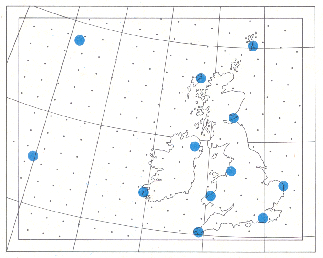
Our new numerical model of the atmosphere predicts meteorological parameters at 10 levels in the atmosphere, and will supersede a simpler model which for several years has been used to prepare daily numerical forecasts of pressure patterns at three levels. These patterns have subsequently been used by human forecasters to infer subjectively the corresponding rainfall distributions. The 10 level model will make available, for the first time in this country, direct computer forecasts of rainfall. In the United States an operational computer model giving direct rainfall forecasts is already in use, but it is not designed to provide the detail given by the new British model. In addition to data about rainfall distribution the computer rainfall forecasts will provide information, never before available, about both distribution and quantity of rainfall to be expected. Both instantaneous rates of rainfall and rainfall accumulations over, say, 24 hour periods will be forecast at each of an array of grid points about 100km apart covering the whole of western Europe and ocean areas. The grid squares are smaller than those of previous computer models of the atmosphere, so that more detail of the variation of weather from one part of Britain to another will be forecast. Another useful feature is that the forecasts will discriminate between the comparatively steady rain at warm and cold fronts and the showery rainfall which results from smaller scale convective motions.
NUMERICAL WEATHER prediction was first carried out by L. F. Richardson who, in his intriguing book Weather prediction by numerical process, published in 1922, described a model atmosphere in which a careful account was taken of all the main physical processes which influence the weather. The model used grid squares with sides of about 200 km, and there were five levels in the vertical. Richardson described how the fundamental partial differential equations which govern atmospheric flow could be approximated by finite difference techniques. It was thus possible to calculate the instantaneous rates of change of each parameter in the model in terms of their distribution in space at a given moment.
Richardson manually calculated the rates of change of pressure, wind, temperature and humidity for a point over central Europe using grid point data derived from observations recorded at 0700 GMT on 20 May 1910. He extrapolated these rates of change over a six hour period, to infer the changes between 0400 and 1000 on that day. The prediction was a conspicuous failure. A change in surface pressure of 1 45 millibars (in System International units one millibar is equivalent to 100 newtons per square metre) during the six hour period was predicted, whereas in reality almost no change occurred. Richardson attributed the errors to inevitable inaccuracies in measuring the initial wind field at upper levels (at that time there were few reliable measurements except at the surface) and believed that sufficient improvements in the observations would enable successful forecasts to be computed using his method. Of course, in that pre-computer age it was impossible to produce a numerical forecast in advance of the actual weather developments; in the preface of his book Richardson wrote, Perhaps some day in the dim future it will be possible to advance the computations faster than the weather advances and at a cost less than the saving to mankind due to the information gained. But that is a dream.
The dream was beginning to come true before Richardson died in 1953. During the mid-1940s J. von Neumann's group at the Advanced Study Institute, Princeton, had built an electronic computer with numerical weather prediction primarily in mind, and from about 1950 onwards increasing research effort was applied to numerical prediction in both Britain and the US. In parallel the necessary improvements in the observational coverage of the atmosphere had been developed, largely stimulated by World War 2, including the widespread adoption of radiosonde techniques whereby instruments are carried aloft by balloons and measurements are returned to the surface by radio.
The methods of numerical weather prediction developed during the 1950s were rather different from Richardson's original proposals. Like his scheme, these methods were based on the calculation of instantaneous rates of change of parameters from knowledge of their spatial distributions, the extrapolation of these rates of change over a certain interval of time (known as the time step) to obtain a new spatial distribution, and the repetition of this process to advance the state of the atmosphere, time step by time step, through a desired forecast period. By now, however, it had become realized that the choice of a particular distance separating the grid points of a numerical model sets a maximum to the time step which may be used; if a longer time step is used, no useful predictions can be obtained. Richardson computed his trial forecast with a single time step of six hours, whereas in fact the critical time step for his model, with a grid separation of some 200 km, was about six minutes.
The fundamental equations which Richardson used - the so-called primitive equations - describe many kinds of atmospheric motion, from fast-moving gravity waves up to the major weather systems. It is well known that for the latter-depressions and anticyclones - the pressure gradient force and the apparent force due to the Earth's rotation are approximately equal and opposite. In 1948 J. Charney, of the Princeton group, showed that it was possible, by careful use of this geostrophic approximation, to derive from the primitive equations what became known as filtered equations which describe only the motion of depressions and anticyclones. Since much longer time steps could be used in filtered models important economies in computing time were possible.
The early filtered models predicted pressure patterns at a single level in the atmosphere. Later, models dealing with two or more levels were developed, but the representation of the atmosphere remained extremely simplified. There was usually no attempt to represent even the effects of moisture in the atmosphere even less to predict rainfall. A three level filtered model has been in daily operational use in the Meteorological Office since 1966.
The much simplified representation of the atmosphere achieved by filtered models has enabled computer forecasts to match the accuracy of traditionally prepared forecasts in predicting the movement and development of the major weather systems. During the past ten years interest has turned towards increasing the amount of detail in numerical forecasts and in particular towards including moisture as a basic parameter of the model atmospheres with a view to predicting rainfall numerically. As a consequence interest has reawakened in the use of the primitive equations, since the assumptions implicit in filtered models are known to be inappropriate in rain producing regions of the atmosphere. The prediction of humidity as an independent parameter, the adoption of shorter grid lengths to provide more detail in the forecasts, and the necessity for shorter time steps in primitive equation models, have all increased the amount of computation required for a forecast of a given period over a given area. Fortunately the technology of electronic computers has also developed to provide the necessary calculating power.
IN 1967 F. H. Bushby and Margaret S Timpson of the Meteorological Office published an account of the first successful 24 hour forecast computed with a 10 level primitive equation model of the atmosphere, and illustrated convincingly the potential accuracy of the rainfall predictions. The model had originally been designed as a research tool for investigating the characteristics of warm and cold fronts, but when it became apparent that such useful rainfall prediction might be achieved, effort was concentrated on developing it for short range rain forecasting. Although some important modifications have been made during the past three years, the model described by Bushby and Timpson is essentially similar to that which will be used operationally on the new computer.
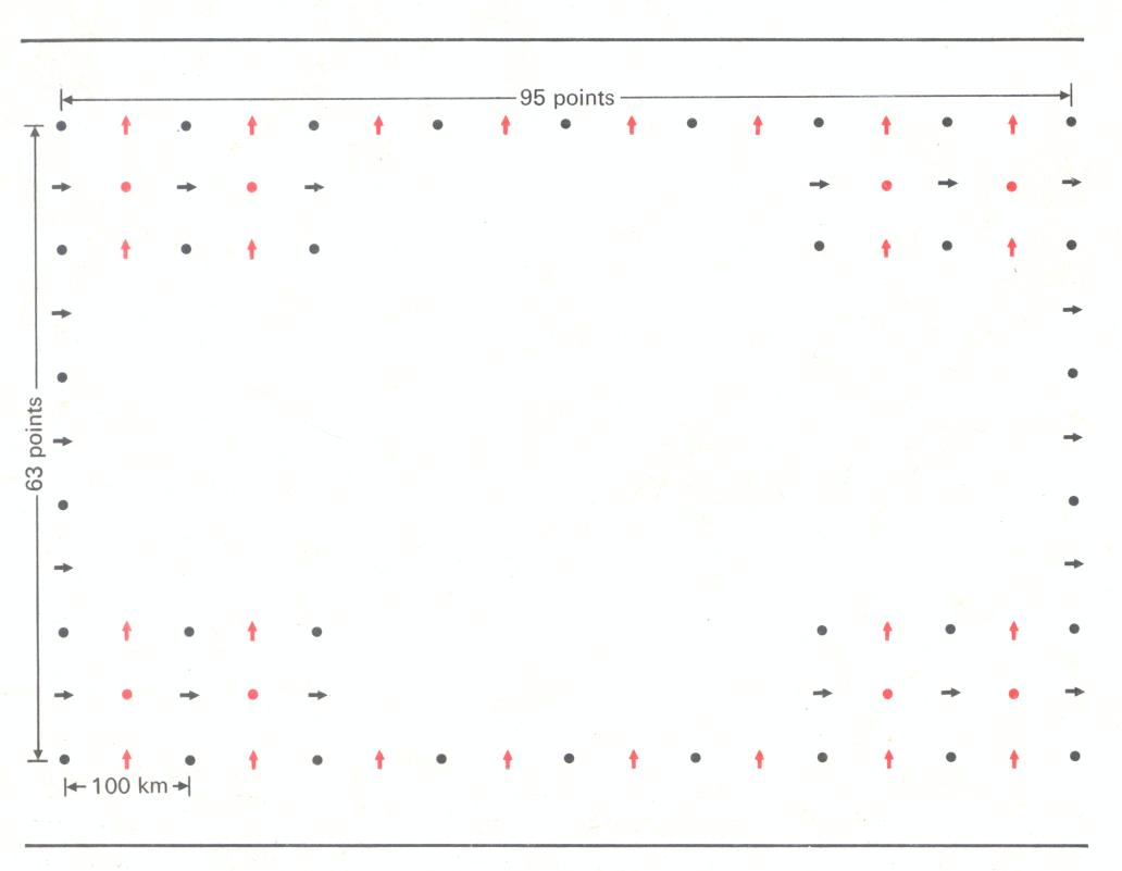
The 10 level model uses pressure instead of altitude as the vertical co-ordinate - a well known device in meteorology which simplifies the equations. The vertical structure of the atmosphere is specified by the heights above mean sea level of 10 surfaces of equal pressure from 1000mb (the approximate pressure at the Earth's surface) at intervals of 100mb down to a pressure of 100mb (at an altitude of approximately 16km). When mean sea level pressure is less than 1000mb the height of the lowest surface is assigned an appropriate negative value. The contour heights of these 10 surfaces are predicted for a grid array which is rectangular on a polar stereographic projection. The finite difference scheme used in the model is such that the contour heights are predicted only at alternate grid points, so that during the development of the model, for example, the heights have been predicted at 48 × 32 points out of a total array of 95 × 63. When the model is used operationally on the new computer a larger array, with some 12,000 grid points, will be employed. The three components of the wind velocity vector are also predicted at the 10 equal pressure surfaces, each one at different grid points, each again at alternate points of the 95 × 63 array.
In each of the 100mb layers below the 300mb level a parameter which specifies the fraction by mass of water vapour in the air, known as the humidity mixing ratio, is predicted at the same grid points as the contour heights. It is assumed that the atmosphere is completely dry above this level. The temperature of the air does not appear as an independent parameter of the model, but a representative temperature of a given 100mb layer may be inferred from the vertical separation of the two bounding equal pressure surfaces, that is, from the thickness of the layer. This is because a 100mb layer of air has fixed mass per unit area, so that warm air, being less dense, occupies a greater volume and therefore corresponds to a greater layer thickness than cool air. The 95 x 63 grid points are spaced at intervals of about 50km over the Earth's surface, but since each parameter is predicted only at alternate grid points there is an effective horizontal resolution of 100km. A time step of three minutes has generally been used for predictions, this being just less than the critical value for a grid length of 100km so that 480 time steps are required for a 24 hour forecast. The large number of grid points used in the model and the number of time steps required indicate the huge amount of computation needed to produce a 24 hour forecast.
THE INITIAL DATA required to begin a forecast are derived from radiosonde observations of the atmosphere at points somewhat irregularly spaced over the Earth's surface. The first task therefore is to analyse these observations and thus obtain the necessary grid point values of contour heights and humidities. During the research stage these analyses were performed manually. In 1968 G. R. R Benwell and M. S. Timpson demonstrated that such an analysis can lead to vertical inconsistencies in the initial data which prevent the successful computation of 24 hour forecasts unless special precautions are taken.
Computer techniques of objective analysis are being developed for use in operational forecasting with the 10 level model, in order that the initial data can be quickly prepared and the forecast commenced. The three components of the initial wind field are obtained from the initial contour height field using equations which describe a state of balance between wind and pressure which approximates to reality. In this way the difficulties encountered by Richardson in attempting to use observed winds as initial data are overcome. As P. W. White of the Meteorological Office described in 1969, progressively more sophisticated treatments of this initial wind problem have been found necessary as the sample of trial forecast dates has been extended.
The rectangular region for which these trial forecasts have been computed has dimensions of about 5000 × 3000km and occupies a portion of the mid-latitude atmosphere. It is in the very nature of the problem that the lateral boundaries of this region cut across the basic atmospheric flow. In the early days of numerical forecasting with this model serious problems were encountered in obtaining any kind of control near these boundaries, but these have been overcome by the introduction of artificially large dissipation effects in these regions. Even so, difficulties remain, because during a forecast period the characteristics of the air flowing across the boundaries of the computational area are constantly changing. Since these changes cannot be simulated-contour heights, winds and humidities being assumed constant on the boundaries-forecasts cannot be regarded as reliable. Even for the central part of the area useful forecasts are usually limited to about 30 hours. The situation will, of course, be improved by the adoption of a larger computational area in the operational model.
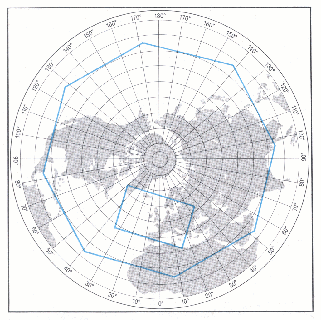
The 10 level model has recently been adapted to compute forecasts over a large octagonal area which includes most of the northern hemisphere. Boundary problems in this area are much less severe since the flow is generally parallel to the boundaries. It is hoped to compute five day forecasts over this area, with a grid spacing three times greater than that for the rectangular area. It might also be possible to use the octagonal model to predict the changes on the boundaries of the rectangular area, thereby extending the useful period of the finer grid rainfall predictions.
THE PHYSICS of clouds and precipitation in the real atmosphere is a complex matter and in the model a much simplified treatment is required. For a given thickness of a particular 100mb layer there is a maximum value - the saturation mixing ratio-above which the humidity mixing ratio is not allowed to rise. If the motion in the model atmosphere is such that the humidity mixing ratio of a layer tends to exceed the saturation value, some of the water vapour is condensed to form liquid water and falls immediately towards the surface as rain. Latent heat is released by the condensation and this warms the air in the layer concerned. If the rain falls through unsaturated air on its way to the surface some of it will evaporate. Originally the model was very drastic in its treatment of rainfall evaporation but recently, in order to improve the accuracy of rainfall distribution predictions near fronts, a more realistic treatment has been devised in which the proportion of the rain which evaporates depends on the rate of rainfall and relative humidity.
The atmosphere as represented in the original model described by Bushby and Timpson was idealized in that it neglected the effects of several important physical processes. Since 1967 extensive research has been devoted to making the model more realistic by incorporating representations of a number of these processes. The influence of friction between the air and the Earth's surface on atmospheric motion has been included, and the effects of cumulus clouds have been represented by vertical heat and moisture transport in appropriate regions of the model atmosphere. This has enabled predictions of convective or showery rainfall to be made. Since shower producing convection is often initiated by heat and moisture transfers from the Earth's surface into the air above, these effects have also been incorporated.
Over the sea the surface temperature is the determining parameter and remains fairly constant in time. Over land however, the exchange of heat and moisture between surface and atmosphere depends on the incoming energy from the Sun, and so the diurnal solar cycle has been taken into account. Since cloud cover has a significant influence on incoming solar radiation, an estimate of cloud amount has been made from the humidities predicted in the model atmosphere. The manner in which the solar energy arriving at the ground is partitioned between heat transfer into the atmosphere and evaporation from the surface depends on soil and vegetation type and on the amount of moisture in the soil. Over deserts virtually all of the solar energy is transferred to the atmosphere in the form of heat, but over well watered grasslands some two-thirds is used up in evaporation. In the model each land grid point is classified according to climatic information, and the balance between heating and evaporation is determined according to climate dependent parameters.
The representations of surface exchanges and cumulus convection incorporated into the model have shown some success in predicting showery rainfall. Difficulties of interpretation arise because of the inherently sub-grid scale nature of such rain. The rainfall amounts predicted in the model represent grid square average values. Since an individual shower occupies only a small part of a grid square, predicted rainfall amounts are much smaller than those which might actually be experienced at individual locations.
Another important factor for rainfall is the effect of hills and mountains on air motion. A representation whereby air at the 1000mb level is forced to ascend on upwind slopes and descend on downwind slopes reproduces a number of realistic effects. However there is again a problem because of sub-grid scale features. Individual hills and peaks cannot be directly represented because they are much smaller than the grid squares but have a significant effect on rainfall. It is evident from a number of the trial forecasts that rainfall amounts predicted over, for example, the Welsh mountains, are often deficient because the full orographic effects are not represented in the model. We are trying to solve this problem.
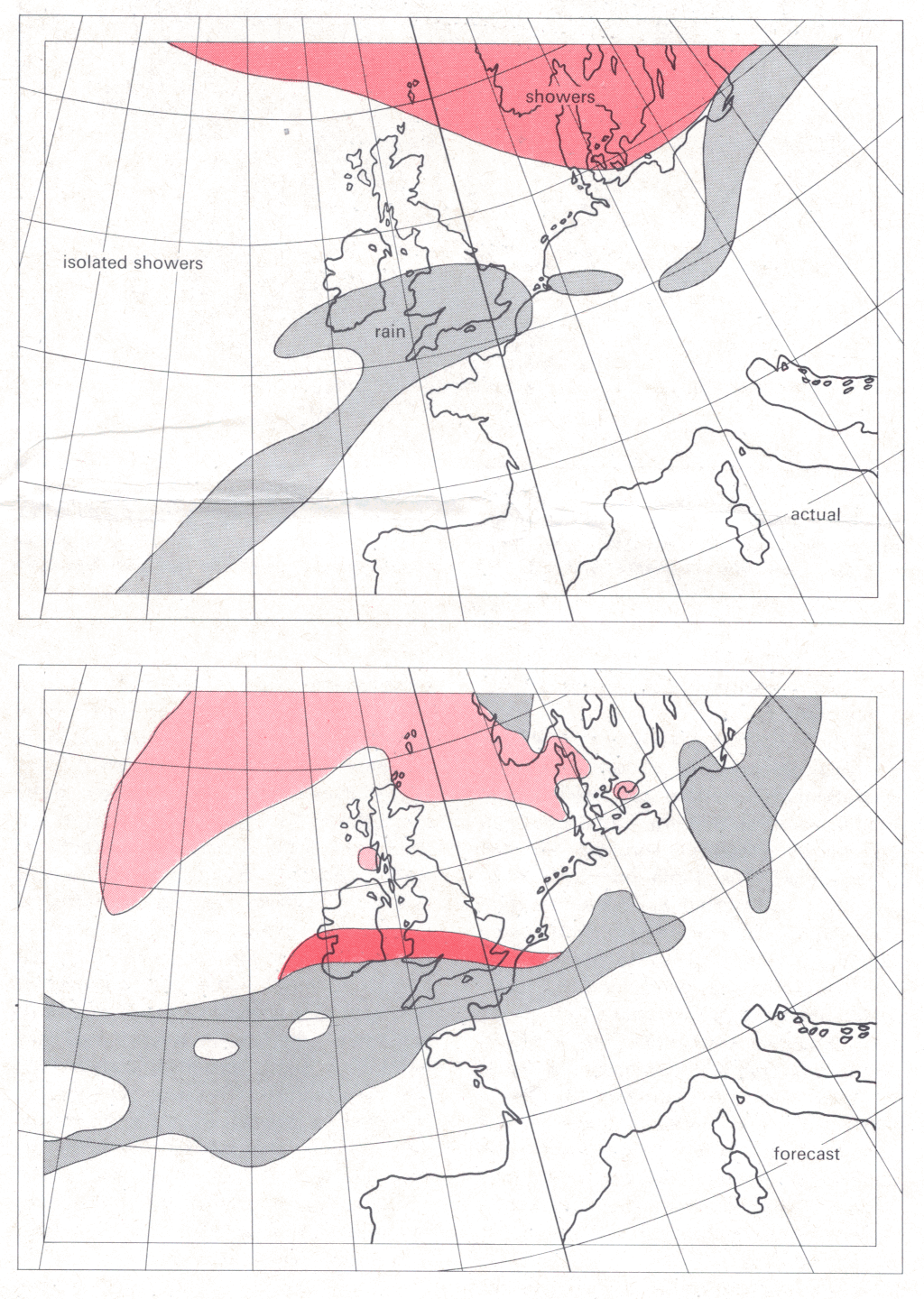
THE OCCASIONS for which trial forecasts have been computed with the 10 level model have been selected either because of some significant weather occurrence, as with two cases of severe flooding in 1968, or because some particular observations have been available. The case illustrated in this article, 16 October 1967, was one for which detailed observations of the structure of a depression were available from a study carried out at the Royal Radar Establishment, Malvern. The 10 level model proved itself capable of reproducing much of the observed structure in this depression.
The results illustrated demonstrate both the great potential of the model and also the current limitations which call for further research. The forecast rainfall distribution at 1200 GMT 16 October 1967 indicates that the 10 level model successfully simulated the advance of a belt of frontal rainfall across the British Isles from the south. The occurrence of showery rainfall, associated with heating from the sea surface, to the north of the British Isles was also correctly predicted. The positioning of the northern edge of the frontal rain belt has been improved by the refinement of the representation of raindrop evaporation in the model. This feature would clearly be important when predicting the time of onset of rain at a given location. It is also evident from this forecast that the fixed parameters on the lateral boundaries have had a detrimental effect in the western part of the area.
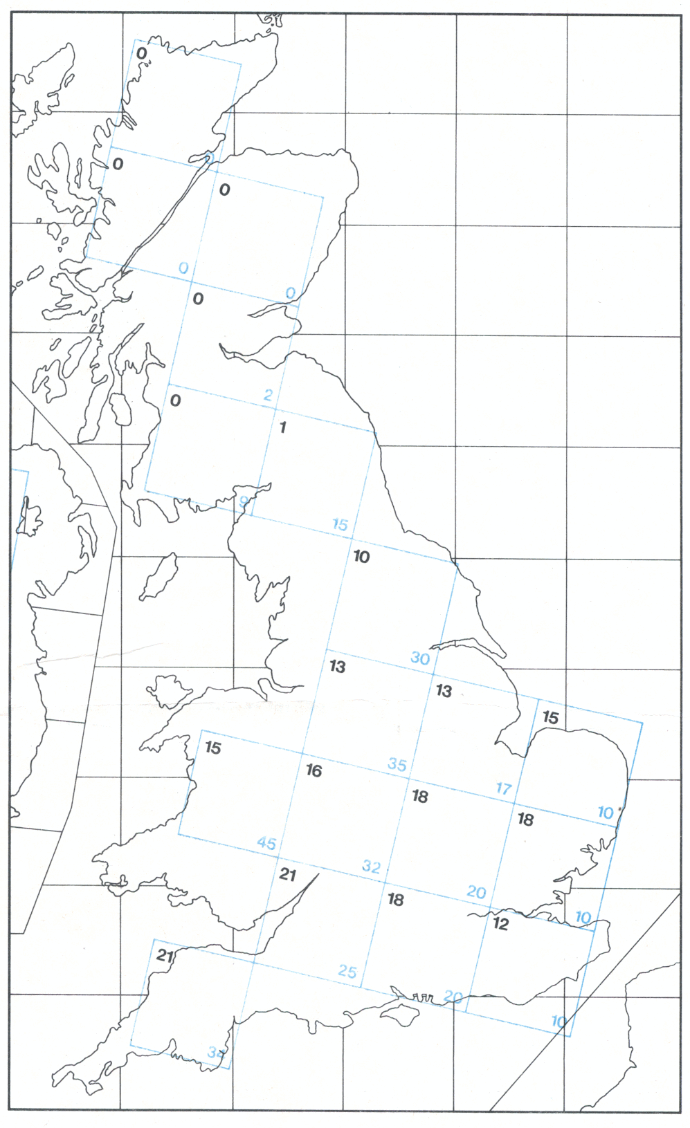
The forecast rain totals for the 24 hour period of 16 October 1967 are in good agreement with actual totals in some areas, but over high ground there are serious deficiencies. Examinations of individual reported totals reveal that on many occasions there are large variations in rainfall accumulation within a grid square. These variations are related to small scale orographic features and small scale atmospheric motion systems which are as yet imperfectly understood. Sub-grid scale features of the rainfall patterns contribute significantly to the actual grid square mean values, but are not represented in the 10 level model.
THE ACQUISITION of computing power sufficient to permit the 10 level model to be used operationally will make available forecasts of the state of the atmosphere up to 1 6km with greater detail than before both in the horizontal and vertical. The greater detail may prove useful in improving existing meteorological services which require, for example, forecast winds or temperatures. However, the essentially new feature will be the prediction of amounts, distribution and times of onset of rainfall. The inclusion of humidity as a basic predicted parameter also opens the way to the eventual forecasting of cloud amount, sunshine, showers and other features which go to make up weather.
Among the research which remains to be done, attempts to devise representations of the full effects of orography on rainfall are very important for the accuracy of predicted rainfall totals. Attention is also being given to modifying the scheme for predicting showery rainfall, since at present the model tends to predict showers when the cumulus clouds would not be of sufficient depth. A further research task is to formulate a representation of the ice-phase so that careful discrimination between rain and snow will be possible. Of considerable importance in the long term is the problem of introducing real boundary changes during the course of a forecast. This will involve the use of models with different grid resolutions with the computational area of one model nested inside that of another. One might envisage that ultimately a hierarchy of several nested models, the coarsest dealing with the whole globe and the finest with just a part of the British Isles, might together be used to deal more directly with small scale features and thus obtain truly local forecasts.
WEATHER PREDICTION BY NUMERICAL PROCESSES by L. F. Richardson (Cambridge University Press, 1922; Dover Publications, 1965)
NUMERICAL WEATHER PREDICTION AND ANALYSIS by P. D. Thompson (MacMillan, New York 1961)
A 10 LEVEL ATMOSPHERIC MODEL AND FRONTAL RAIN by F. H. Bushby and Margaret S. Timpson {in Quarterly Journal of the Royal Meteorological Society, 93, 395, 1967)
NUMERICAL WEATHER PREDICATION by (B. J. Mason (in Report on the Culham Computational Physics Conference, HMSO London, 1969)
NUMERICAL WEATHER PREDICTION USING A 10 LEVEL ATMOSPHERIC MODEL by G. R. R. Benwell (in Bulletin of the Institute of Mathematics and its Applications, 6, 56, 1970)
