
A set of high level subroutines for the drawing of curves, histograms etc, the hatching of areas and three-to-two dimensional projection is accessible to the SMOG package and they are described here for completeness.
2-D Routines
Histograms
  HSTGMA                         Single shaded histogram
  CMHSTA                         Composite shaded histogram
Shading
  TXTURA                         Shading rectangular area
Curve Drawing
  CVFNCA
  CVFNCB                         Single valued function plot
  CVFNCR
  CVFNCS
  ARCA
  ARCB                           Arc of a circle
  ARCR
  ARCS
  CIRCLA
  CIRCLB                         Complete circle
  CIRCLR
  CIRCLS
  ELLPSA
  ELLPSB                         Complete ellipse
  ELLPSR
  ELLPSS
Miscellaneous
  AROWHR                         Arrow heads
  AROWVR
  BOXA                           Rectangle
  BOXR
Graphs
  GRAPH                          Draw complete graph
  GRAFT                          Draw graph with options
  GRAFRG                         Make region suitable for graphs
  TITLAB                         Draw titles and labels
  SCALA                          Draw scales
  AXESA                          Draw axes
3-D Projection Routines
  ZVIEW                          Defines the projection plane
  ZVIS                           Defines "Side" of plane
  SETXYZ                         Absolute "Set"
  TOXYZ                          Absolute "Draw"
  UPDXYZ                         Relative "set"
  TODXYZ                         Relative "Draw"

  VECZ                           "3-vector" projection
  HPLOTZ                         Plot character
  EXPANZ                         Expand about a point

  ROTXZ                          Set axis for rotation
  ROTANZ                         Set angle of rotation

  ERDRZ                          Defines order: expansion/rotation

  CUBER                          Projects cube onto plane
      ARCA(X,Y,RAD,D,THST,THFI,P)
      ARCB(X,Y,RAD,Q,THST,THFI,P)
      ARCA(RAD,D,THST,THFI,P)
      ARCB(RAD,Q,THST,THFI,P)
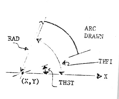
draw an arc of a circle of radius RAD.
ARCA, ARCB take the circle's centre to be (X,Y) and draw an arc from THST to THFI using VEC orders. ARCR,ARCS start the arc at the current, plotting position and use Relative orders (ie the centre of the circle is assumed to be (XP-RAD*COS(THST),YP-RAD*SIN(THST)). (See Section 4.2.) In ARCA,ARCR, each line segment of the arc is less than D in length. In ARCB,ARCS, Q equal line segments are used. If P=0.0, all lines are drawn, otherwise only every other line is visible, giving a dotted arc. The end-point of the arc will be the current plotting position on exit.
Possible errors are the same as for the circle drawing routines (9.1.6, 9.1.7) (qv).
      AROWHR(DX,DY)
      AROWVR(DX,DY)
each draws an arrow head (V) at the current plotting position the size of which is given by DX,DY. AROWHR draws a horizontal arrow (left if DX positive, right if DX negative). AROWVR draws a vertical arrow (up if DY positive, down if DY negative).
BOXA(X1,Y1,X2,Y2)
BOXR(DX,DY)
draw rectangles. BOXA uses VEC orders and constructs the rectangle so that the bottom left-hand corner is (X1,Y1) and the top right-hand corner is (X2,Y2), leaving the current plotting position at (X1,Y1). BOXR uses relative orders and, starting from the current position, constructs the rectangle with sides DX,DY.
      CIRCLA(XX,YY,RAD,D,P)
      CIRCLB(XX,YY,RAD,Q,P)
      CIRCLR(RAD,D,P)
      CIRCLS(RAD,Q,P)
draw a circle of radius RAD.
CIRCLA,CIRCLE select (XX,YY) as centre and use VEC orders. CIRCLR,CIRCLS select the current plotting position as centre and use relative orders. The centre will be the current plotting position on exit. CIRCLA, CIRCLR construct the circle so that each line segment is less than D in length. CIRCLE,CIRCLS construct the circle from Q lines of equal length. If P = 0.0, all lines are drawn, otherwise only every other line is visible, giving a dotted circle.
The following errors are possible:
RAD<0.0        ABS (RAD) taken, or 1.0 if RAD = 0.0
D<0.001*RAD    D = 0.1*RAD
Q<1.0          ABS (Q) taken, or 8.0 if Q = 0.0
CMHSTA(XMN,YMN,DELTAX,DYAR,YMAX,CMAX,DX,DY,TYPE,SRND)
this subroutine is similar to HSTGMA (9.1.13) but produces a composite histogram. All the Y values involved are contained in the single dimensioned array DYAR. It is recommended that the user sets up the Y values in a two dimensional array whose limits are YMAX,CMAX and then uses the EQUIVALENCE statement to provide the single dimensioned array needed for the argument to this routine. For example:
      DIMENSION DZ(YMAX,CMAX),DYAR(YMAX*CMAX)
      EQUIVALENCE (DZ(1,1),DYAR(1))
Each histogram in this example should be contained in DZ(1,N) to DZ(YMAX,N). TYPE is a single dimension array, specifying the type for each histogram in the set. Similarly, DX,DY are single dimension arrays. Any negative Y values encountered in a histogram are taken to be zero.
      CVFNCA(F,XMN,XMX,DX,DY)
      CVFNCB(F,XMN,XMX,P)
      CVFNCR(F,XMN,XMX,DX,DY)
      CVFNCS(F,XMN,XMX,P)
draw the curve Y=F(X) between the X values XMN and XMX. F(X) must be a single-valued real function in the range. The curve is drawn using either VEC orders (CVFNCA,CVFNCB) or TODXY orders (CVFNCR,CVFNCS). If DX,DY are specified, the curve is drawn so that each line segment has an X-increment less than or equal to DX and a Y-increment less than or equal to DY. If P is specified, the curve is drawn using P lines, equally spaced in the X direction.
The following errors can occur:
XMX<XMN          curve drawn from XMX to XMN
XMX-XMN>100*DX   DX = 0.1*(XMX-XMN)
DY≤0             DY = 1.0
P<0              MOD (P) taken
P=0              P = 1.0
      ELLPSA(XX,YY,A,B,DX,DY,P)
      ELLPSB(XX,YY,A,B,Q,P)
      ELLPSR(A,B,DX,DY,P)
      ELLPSS(A,B,Q,P)
draw an ellipse whose major and minor axes (parallel to X,Y axes) are A,B respectively. ELLPSA, ELLPSB select (XX,YY) as centre and use VEC orders. ELLPSR,ELLPSS select the current position as centre and use relative orders. The centre will be the current plotting position on exit. ELLPSA,ELLPSR construct the ellipse so that each line segment has X,Y increments less than DX,DY. ELLPSB,ELLPSS construct the ellipse from Q lines, subtending equal angles at the centre. If P=0.0, all lines are drawn, otherwise only every other line is visible.
Possible errrors are:
A,B<0.0         Absolute value taken, or 1 if zero
DX<.001*A       DX = 0.1*A
DY<.001*B       DY = 0.1*B
Q≤0.0           Absolute value taken, or 8 if zero
HSTGMA(XMN,YMN,DELTAX,DYAR,YMAX,DX,DY,TYPE,SRND)
produces a histogram with the interval in the X direction = DELTAX. The origin is assumed at (XMN,YMN). The Y values are contained in array DYAR (I) where I = 1,YMAX. TYPE defines the pattern used in the histogram, as given in TXTURA. SRND =0.0 draws a border around the histogram but excluding the baseline. SRND = 1.0 will draw the baseline as well. Any errors are processed by TXTURA.
TXTURA(XMN,YMN,XMX,YMX,DX,DY,TYPE,SRND)
the subroutine TXTURA puts a pattern on the rectangular area having opposite corners (XMN,YMN) and (XMX,YMX). The pattern is defined by the parameter TYPE with parameters DX,DY defining the period. SRND specifies whether or not the border surrounding the area is drawn (SRND = 0.0 for no border, SRND = 1.0 for border).
The possible values of TYPE are:
 0.0  no pattern
 1.0  horizontal lines, DY apart
 2.0  vertical lines, DX apart
 3.0  combination of 1 and 2
 4.0  diagonal lines, angle to horizontal THETA where TAN(THETA) = DY/DX
 5.0  diagonal lines, angle to horizontal THETA where TAN(π-THETA) = DY/DX
 6.0  combination of 4 and 5
 7.0  horizontal dashed lines, DX long, DY apart
 8.0  as above, but every other line displaced by DX
 9.0  vertical dashed lines, DY long, DX apart
10.0  as above but every other line displaced by DY
Parameters not used for a particular value of TYPE should be set to 0.0.
NB Types 1, 2 and 3 can be obtained more efficiently by using vector family orders (4.1.10, 4.1.11).
The following errors can occur:
XMX<XMN          Routine takes no action
YMX<YMN          Routine takes no action
DX<0             MOD (DX) taken
DY<0             MOD (DY) taken
XMX-XMN>500*DX   DX = .002*(XMX-XMN)
YMX-YMN>500*DY   DY = .002*(YMX-YMN)
Several routines have been provided to assist the user in drawing graphs, labelling axes, etc. The first provides a 'standard' graph making various assumptions. The second allows the user to vary the type of labelling, tick marks, etc. Others merely draw axes or scale them.
GRAPH(N,XAR,YAR,NT,TITLE,NX,XLABEL,NY,YLABEL)
N        Number of points for graph, the dimension of arrays XAR,YAR.
XAR      Single dimensioned arrays giving the X,Y coordinates of the
YAR      N points making the graph.  Straight lines will be drawn
         between consecutive points.
NT       Number of characters to appear in the title.
TITLE    Text for title, either as a text constant or first element of
         an array containing packed text. The title will appear above
         the graph.
NX       Number of characters to appear in the X axis label.
XLABEL   Text for X axis label in the same form as TITLE.  The label will
         appear below the scaling values on the axis.
NY       Count and text for Y axis label, which will appear to the left
YLABEL   of the scaling values on the Y axis.
GRAPH will find the maximum and minimum values in arrays XAR,YAR, and scale the graph so that it fills as much of the area as possible. Axes, major and minor tick marks are provided, and scale values printed at the major tick positions. The number of major tick marks depends on the values being scaled, Ten minor ticks appear between each major tick. F format is used if the numbers lie in the range ±0.0001 to 100000.0, otherwise E format is used for the scale values.
Example
      MASTER XX
      DIMENSION ARX(100),ARY(100),TITLE(4)
      DATA TITLE(1)/22H THIS GRAPH HAS A TITLE/
C     values for ARX.ARY
      CALL FRHCM
      CALL GRAPH(100,ARX,ARY,22,TITLE(1),16,
     *'HORIZONTAL LABEL',14,'VERTICAL LABEL')
      CALL ADVFLM
      CALL ENDSPR
GRAFT(I,N,XAR,YAR,GRAT,FORM,APLOT)
I       Option indicator. The various options available are described  below.
N
XAR     Count and arrays of points for graph, as for routine GRAPH.
YAR
GRAT    Graticule/tick indicator.
        0.0 No graticules or tick marks
        1.0 Tick marks, major divisions only
        2.0 Tick marks, major and minor divisions
        4.0 Major graticule markings
        8.0 Major and minor graticule markings
        Graticules will extend over the whole graph.  Any combination
        of the above may be used (for example, 5.0 will cause major
        tick marks and major graticules to be drawn). Number of major
        ticks or graticules depends on the values being scaled
        (usually between 5 and 15 major marks are used).
        There are 10 minor divisions between each major division.

FORM    Scale value format, tick mark control
        0.0 Scales printed in E or F format (see GRAPH)
        1.0 Scales printed in I format
        2.0 No axis, tick marks or scaling for X
        4.0 No axis, tick marks or scaling for Y
        8.0 Y axis and scales left shifted for second graph
        Any combination of these values may be used.  Option 8.0 should
        be used with option 2.0, ie [10.0], FORM does not override GRAT
        if graticules are requested. Scale values, when printed, are
        drawn outside the current region (see 9.2.4).
APLOT   Graph format.
        1.0 to 64.0 (option 1, 2 or 4).  Graph plotted as separate points
        using the character defined by number APLOT (see 5.1.1).
        0.0  Graph plotted as continuous line.
        (option 3 or 5). Axes, scales, etc, are to be saved in file
        number APLOT using FRSAV (see 7.1.1).  No graph will be plotted.
The possible optional values of I are:
I=1,2   Scale the graph according to maximum and minimum values obtained
        from arrays XAR, YAR.  Reset the current region limits accordingly.
        Draw tick marks, scales, etc, according to parameter settings.
        Draw graph.
I=3     Calculate scales, etc, as for option 2,  However, rather than drawing
        a graph, save the axes, scales, etc, in the file specified by APLOT
        parameter.
I=4     Use the current region limits to determine the required
        scales.  Draw tick marks, etc, according to parameter settings. Draw graph.
I=5     As for option 4, but save the axes, scales, etc, in the file specified
        by APLOT parameter.
In each case, the current region is taken to contain the whole graph. Axes are drawn along the region edges and scales are printed outside the region boundary.
Multiple graphs can be drawn on the same grid by using the parameters:
   GRAT = 0.0
   FORM = 6.0
which prevent the re-drawing of scales, axes, etc, or by drawing the lines in the normal way, for example:
      CALL SETXY(XAR(1),YAR(1))
      DO 10 I=2,N
  10  CALL TOXY(XAR(I),YAR(I))
If a second Y axis labelling scheme is required, use can be made of parameter:
FORM = 10.0
which provides a scaled Y axis to the left of the normal position. The region (and therefore graph) limits can be recalculated or left the same by using option 2 or 4.
TITLAB(NT,TITLE,NX,XLABEL,NY,YLABEL)
draws titles and labels where the arguments are the same as those in GRAPH. Titles and labels are also printed outside the current region boundary, and TITLAB should be called after a call to GRAFT. It does mean, however, that the current region must map into an area which occupies less than the whole screen.
GRAFRG(1.0)
defines region 1 for drawing the graphs, scales, etc. The region has the same limits after the call as it had before but maps into approximately 0.75 of the previous area leaving a border around the edges. The border at the top is used for the title, that to the left for the Y axis scale and label and that at the bottom for the X axis scales and label.
GRAFRG(-1.0)
is the inverse of GRAFRG(1.0). It resets the plotting area to that prior to the call to GRAFRG(1.0).
A call to GRAPH is equivalent to the following:
      CALL GRAFRG(1.0)
      CALL GRAFT(1,N,XAR,YAR,2.0,0.0,0.0)
      CALL TITLAB (NT,TITLE,NX,XLABEL,NY,YLABEL)
      CALL GRAFRG(-1.0)
Example
Draw two graphs, the first using the limits provided and the second using limits calculated from the data. The second graph also has graticules.
      CALL FRHCS
      CALL CINE
      CALL LIMITS(0.0,0.0,100.0,100.0,1.0,1.0)
      CALL GRAFRG(1.0)
      CALL GRAFT(4,100,XAR,YAR,0.0,1.0,0.0)
      CALL TITLAB(    ....    )
      CALL ADVFLM
      CALL GRAFT(2,100,XAR,YAR,8.0,1.0,0.0)
      CALL TITLAB(    ....    )
      CALL GRAFRG(-1.0)
      CALL ENDSPR
SCALA(DX,DY,X,Y,XI,XJ,YI,YJ)
labels the axes taking (X,Y) as the origin. Values are printed below the X axis, DX apart, and to the left of the Y axis, DY apart, to the edges of the region. If either DX or DY is zero, that particular axis will not be scaled. On exit, the current plotting position will be (X,Y). XI,XJ and YI,YJ define the formats of the numbers printed in the X and Y directions respectively. (See definition of TYPNMB (5.2.9) for possible formats).
AXESA(X,Y)
draws axes through (X,Y), reaching to the edges of the region, the current plotting position will be (X,Y).
The following routines provide a projection onto the output medium (the "View Plane") of a set of triples (Xi,Yi,Zi) which could, for example, be points on the surface f(X,Y,Z)=0. The projection is in perspective from the point of view of the viewer, situated "D" units along a normal to the view plane. The routines use standard SMOG routines and so the resulting plotting orders may be saved in the normal way (see Section 7). The diagram illustrates the process.

The boundary to the visible area in the view plane is set as in Section 3 and similar scaling applies.
There is an error in this figure. The axis marked X should be Z and the one marked Z should be Y
ZVIEW(XV,YV,ZV,D)
defines the location of the viewer (XV,YV,ZV) and the distance, D, from the viewer to the view plane in the direction of the origin. D may be negative. The viewer always looks towards the view plane and anything behind him will be hidden. There is no hidden line removal in the object itself.
The view plane may cut the object being viewed. The routine:
ZVIS(XI,XO)
will set the intensity level of all lines between the viewer and the plane to XI, and the intensity level of all lines on the other side of the view plane to XO. It is thus possible to obscure one or other of the sections by setting the appropriate intensity to zero.
The current 3D position can be moved by:
      SETXYX(X,Y,Z)
      UPDXYX(DX,DY,DZ)
lines can be drawn by:
      TODXYZ(DX,DY,DZ)
      TOXYZ(X,Y,Z)
      VECZ(X1,Y1,Z1,X2,Y2,Z2)
which are all obvious extensions of the 2D routines. 2D routines may be mixed with 3D routines, but the 3D routines will always reset the 2D current plotting position (XP,YP).
Characters can be drawn by:
HPLOTZ('S')
plots the one element character string 'S' at the current 3D position. The character is always drawn in the plane of the screen at the currently selected character size (5.3.6). 3D rotation and expansion have no effect on the actual character but may change its position.
3D expansion is performed by:
EXPANZ(X,Y,Z,EX,EY,EZ)
where EX,EY and EZ are the expansion factors for the X,Y and Z directions.
Rotation about a general axis is performed by two routines:
ROTAXZ(X1,Y1,Z1,X2,Y2,Z2)
which defines the axis of rotation and:
ROTANZ(TH)
which defines the angle (in radians).
The order of expansion/rotation is determined by:
ERDRZ(X)
where:
X = 1.0 means rotation is performed first
X = 2.0 means expansion is performed first
The high level routine:
CUBER(DX,DY,DZ)
will project a cube drawn from the current 3-D point with sides parallel to the respective axes, lengths DX,DY,DZ.
Example
C***ROTATION OF CUBE
      CALL FRHCM
      CALL LIMIT(-3.0,-3.0,3.0,3.0)
      CALL ZVIEW(0.0,0.0,20.0,25,0)
      CALL ROTAXZ(0.0,0.0,0.0,0.0,1.0,0.0)
      TH = 0.0
      STP = 0.31415926
      DO 10 I = 1,6
      CALL ROTANZ(TH)
      CALL SETXYZ(-1.0,-1.0,-1.0)
      CALL CUBER(3.0,3.0,3.0)
      CALL ADVFLM
 10   TH = TH + STP
      CALL ENDSPR
