This paper describes a package for drawing complex three-dimensional objects. Input consists of concave or convex polygons. However, a number of high-level routines shield the user from the details of how objects are defined. Output can be either line drawings, shaded raster lines or three-dimensional contour plots. The package was produced by Michael J Archuleta of Livermore and is a development of the work of Gary Watkins at the University of Utah. The low-level routines have been rewritten so that the package sits on top of either SMOG or SPROGS on the 1906A. The current version is an interim release which will be enhanced and made more efficient if the frequency of use demands it.
The Watkins algorithm accepts as input. convex or concave polygons whose coordinates are defined in a left-handed coordinate system. Polygon clipping is performed to a frustum of vision that opens out along the positive Z axis. The algorithm assumes that the eyepoint is located at the origin of the system. All 3-dimensional polygons are projected onto a 2-dimensional plane. The projection plane is divided into horizontal raster-lines and the algorithm computes the visibility of the polygons a raster-line at a time. A segment (the portion of the raster-line which intersects the polygon) is sorted and compared with other segments to see which are visible.
One drawback of the Watkins' algorithm is that adjacent polygons had to store the shared edge twice. Archuleta has modified the algorithm to allow shared edges to be defined. It is possible to choose whether or not to display shared edges. This is useful when contour plots are required as it stops the confusion between edges and contour lines.
The package contains a number of routines which allow the user to display a surface. The routines are similar in that all define the Z-values of the surface on a two-dimensional X, Y grid of points. If the surface is displayed as a line drawing then neighbouring points in the X and Y directions will be connected by lines. The main difference between individual routines is in the way the grid is defined.
Each type of output is defined by two routines. The first, which ends with the letter I defines the surface as a set of polygons and forms the relevant data structure, The second, which ends with the letter D, displays the surface in the form given by the arguments. For any surface it is only necessary to call the I routine once, The D routine may be called a number of times. The surface may be displayed in a variety of forms and any particular orientation.
A set of routines is provided for translating and rotating the surface before displaying it.
Before a surface can be defined, it is necessary to set up two COMMON blocks and initialise the size of the data base. All routines in the system have the COMMON blocks defined as a minimal size so that the one defined in the user program specifics the size of the data base area. The sizes of these areas are given to the system by calling the routine INFREE which should be the first routine in the package that is called. The necessary declarations are:
       COMMON/FREE/IFREE(2,i)
       COMMON/BUCKY/IB(j)
       CALL INFREE (i,j)
The parameter i defines the free storage working area used by the hidden line routines. It should be set equal to at least 44 times the number of squares that will be plotted if contours are not required and about 52 times the number of squares if contours are to be plotted. Each edge requires either 11 or 13 words depending on whether contours are defined.
The parameter j defines the resolvability of the line drawing device to be used. It is quite sensible to define a low value (say 32) while debugging is being done. The maximum value allowed for j is 1024. A reasonable approximation to the surface is obtained by setting j to 512.
To define a surface consisting of a 20 by 20 grid of squares and not requiring contours would require:
      COMMON/FREE/IFREE(2,17600)
      COMMON/BUCKY/IB(512)
      CALL INFREE(17600,512)
All the high level routines other than WEB require the above COMMON blocks to be set up.
GSURFI(RX2,INFB,INFE,INFD,RY2,INSB,INSE,INSD,RZ2,MAX)
GSURFD(RX2,INFB,INFE,INFD,RY2,INSB,INSE,INSD,RZ2,MAX,I,A)
The arguments are defined as follows:
The arguments given above allow a subset of the array to be used to define the surface. This can be of considerable value during debugging. The coordinates of points on the surface are given by:
      DO 20 I = INFB,INFE,INFD
      DO 10 J = INSB,INSE,INSD
      X = RX2(I,J)
      Y = RY2(I,J)
      Z = RZ2(I,J)
The values of INFB etc should be consistent with their appearance in DO statements of the type given above.
The last two parameters of GSURFD define the type of output and the angle of view. These are described in Section 2.9.
RSURFI(RX1,INFB,INFE,INFD,RY1,INSB,INSE,INSD,RZ2,MAX)
RSURFD RX1,INFB,INFE,INFD,RY1,INSB,INSE,INSD,RZ2,MAX,I,A)
This routine displays a surface consisting of a mesh defined by the arrays RX1 and RY1 and the z-values contained in RZ2. The arguments are defined as follows:
The set of coordinates for points for the surface are given by:
      DO 20 I= INFB,INFE,INFD
      DO 10 J= INSB,INSE,INSD
      X = RX1(I)
      Y = RY1(J)
      Z = RZ2(I,J)
ESURFI(INFB,INFE,INFD,INSB,INSE,INSD,RZ2,MAX)
ESURFD(INFB,INFE,INFD,INSB,INSE,INSD,RZ2,MAX,I,A)
This routine displays a surface where the z-values are defined by the two-dimensional array RZ2. The mesh is an equally spaced grid defined by the arguments which have a similar meaning to those used in GSURF.
The coordinates of the points on the surface are given by:
      DO 20 I= INFB,INFE,INFD
      DO 10 J= INSB,INSE,INSD
      X = I
      Y = J
      Z = RZ2(I,J)
FSURFI(XMIN,XMAX,INXS,YMIN,YMAX,INYS,FRZ)
FSURFD(XMIN,XMAX,INXS,YMIN,YMAX,INYS,FRZ,I,A)
This routine displays a surface where the z-values are defined by the function FRZ. The variables are:
The two parameters I and A are the same as for GSURF.
PATCHI(NPOLY,IPOLY,NPTS,XYZ)
PATCHD(NPOLY,IPOLY,NPTS,XYZ,I,A)
This routine displays a number of polygons defined by the arguments. These are:
COUNT,PT1,PT2, ...COUNT,PT1,PT 2,...For example, if. IPOLY contains:
4,1,2,3,4,3,5,6,2This defines two polygons. The first has four sides and its vertices are defined by the positons l, 2, 3 and 4 in XYZ. The second polygon has three sides and its vertices are defined by the positions 5, 6 and 2 in XYZ. Thus the two polygons have one point in common.
The two arguments I and A are the same as for GSURF.
WEBI(NPTS,XYZ)
WEBI(NPTS,XYZ,I,A)
This routine displays a picture consisting of a set of lines. No hidden line removal is attempted so the COMMON blocks defined in Section 2.2 need not be defined. Also, it is not necessary to call INFREE. The picture is scaled so that the x and y values are in the range -1 to 1. The arguments are:
In the routines given above, the two arguments I and A define the type of output to be generated and the angle of view.
The possible values for I are:
The resolution of the picture is determined by the COMMON block BUCKY and the second argument of the call to INFREE. If this is defined as MAXRAS then the coordinates of the picture will range from 0 to MAXRAS in the x and y directions. By calling:
CALL LIMITS(0.,0.,MAXRAS,MAXRAS,1.,1.)
in SMOG, the complete picture should be plotted.
The parameter A defines the cone of vision in degrees. It may vary between 5° and 120°. Values outside this range will be reset to 45°. If a negative value of A is given, the picture will be displayed as a set of 10 equally spaced contour bands from the minimum Z to the maximum Z of the data specified.
Once an initialisation routine, such as GSURFI, has been defined, it is possible to transform the surface by calling one of the routines given below.
CXROT (R)
Rotates about the x axis by R degrees
CYROT(R)
Rotates about the y axis by R degrees
CZROT (R)
Rotates about the z axis by R degrees
CTRAN(A,B,C)
Translates the surface by A, B and C units. The new coordinates on the surface (X',Y',Z') are defined as:
X' = X+A
Y' = Y+B
Z' = Z+C
CSCAL(A,B,C)
Scales the surface by A,B,C. The new coordinates are:
X' = X*A
Y' = Y*B
Z' = Z*C
CINIT
Resets the transformation to the initial view of the surface.
The intermediate level routines provide the user with more flexibility in the way he defines objects. It is assumed that the user has performed all the necessary transformations to place his data in the desired position for viewing. The information about the objects to be displayed is passed to the system one polygon at a time with the relevant information set up in COMMON blocks.
Initialisation takes place in two stages. First, the data base must be initialised by calling INFREE. This is described in detail in Section 2.2. Once this has been done, several parameters of the system need to be set up before calling INTCLP which verifies that the values given are reasonable and then initialises the hidden line algorithm.
The variables to be defined are given by the following COMMON blocks.
COMMON/CONLEV/CONHI,CONLO,NCONLV,CLEVEL(i)
COMMON/ZRANGE/ZMIN,ZMAX
COMMON/INTENS/IHI,ILO,IBACK,IFRAMX,IFRAMY
The subroutine INTCLP has no arguments. It should be called before any data is passed. It initialises polygon clipper. A typical initialisation sequence might be:
      COMMON/FREE/IFREE(2,8000)
      COMMON/BUCKY/IB(512)
      COMMON/CONLEV/CONHI,CONLO,NCONLV,CLEVEL(10)
      COMMON/ZRANGE/ZMIN,ZMAX
      COMMON/INTENS/IHI,ILO,IBACK,IFRAMX,IFRAMY
      CALL INFREE (8000,512)
      IFRAMX = 512
      IFRAMY = 512
      IHI= 30
      ILO = 6
      IBACK = 3
      XMIN = 10.0
      ZMAX = 60.0
      NCONLV = 10
      CONLO = 1.0
      CONHI = 10.0
      DO 1 I=1,10
      CLEVEL(I) = I
 1    CONTINUE
      CALL INTCLP
      CALL FRHCM
      CALL LIMITS (0,,0,512.,512.,1.,1.)
Once INTCLP has been called, the individual polygons may be passed to the hidden surface algorithm by one of the routines POLSMO or POLCLP. The information defining the polygon must be entered in the COMMON block POLDAT which is defined as:
      COMMON/POLDAT/IEDG,NTERNL,X(12),Y(12),Z(12),SHADE(12),
     1KOLOR(12),CONTUR(12),ISHR(12)
      LOGICAL NTERNL,ISHR
The variables are defined as follows:
POLCLP
The information provided in the array SHADE will be ignored. The remaining information in POLDAT will be used to define a polygon which is clipped and stored for picture processing. The shading for the polygon will be set up automatically using a cosine squared relation with a planar light source located at the z = 0 plane.
POLSHO
This is similar to POLCLP except that the polygon will be defined with the shading information given in SHADE.
POLDIR(I)
This subroutine can be used to find out the position o[ the polygon in POLDAT with respect to the current parameters. It returns a value of 1 if the polygon is clockwise, 0 if it is counter-clockwise and -1 if the polygon has any portion in the negative z-space.
This information is useful if the user has taken care to orient his data. For example, a sphere can be defined by polygons which are all drawn in a 'clockwise' direction. By calling POLDIR, it is possible to find out which polygons are currently on the back side of the sphere (these will be counter-clockwise), It would not then be necessary to pass these to the hidden surface algorithm and thus cut down on the total amount of processing required.
Once all the polygons making up the picture have been defined, the picture can be displayed in a number of different ways by calling the subroutine HIDDEN. This routine has no arguments. The type of output is defined by the current settings in the COMMON block QFORIO which is defined as:
      COMMON/QFORIO/CONTRS,IDVICE,IBAD,SHOSHR,LBLSPC
      LOGICAL CONTRS,IBAD,SHOSHR
The variables are defined as:
For example, to generate a line drawing with no contours but having visible shared edges would require:
      CONTRS = .FALSE.
      IDVICE = 1
      SHOSHR = .TRUE.
      CALL HIDDEN
The user must have set up the MOG or SPROGS initialisation routines prior to calling HIDDEN.
The simplest method of shading an object is to use the routine POLCLP to define the shading. If the user wishes to apply his own shading information then this must be defined prior to calling the routine POLSMO.
The easiest way to shade an object is to assign some arbitrary intensities to the faces of the object. This will ensure that the faces stand out but there will be no obvious light source.
To get realistic shading it is best to define a light source and assume that the object is reflecting light. If A1, B1 and C1 are the constants of the planar equation for the plane which is reflecting light and A2, B2, C2 are the constants for the planar equation representing a planar light source, a cosine shading rule would give:
      SHADE= (A1*A2+B1*B"+C1*C2)/
             (SQRT (A1*A1+B1*B1+C1*C1)*SQRT (A2*A2+B2*B2+C2*C2))
If the planar light source is located on the Z=0 plane, and a cosine squared rule is used:
SHADE= C1*C1 / (A1*A1+B1*B1+C1*C1)
This produces a relatively pleasing picture. To allow shading as a function of distance, it is necessary to divide the value given above by the distance suitably normalised. For example:
SHADE= SHADE/R
where R represents the distance from the light source to a point on the plane. It is important to remember that the SHADE values must lie within the range 0. to 1. and to get best effect the whole of the range should be used. This squeezes as much information out of the picture as possible. However, if a film is being generated, the normalisation must be consistent for all the frames otherwise the object will start to blink!
If a point light source is required at the origin and intensity is defined using a cosine-squared-over-range relation, it is necessary to define the shade values at the two ends of an edge. If the edge has the two end points (XB,YB,ZB) and (XE,YE,ZE) and CX,CY,CZ are the constants defining the plane, then the shading values at the vertices would be SB and SE where:
      CONSTS = CX*CX+CY*CY+CZ*CZ
      CB     = XB*XB+YB*YB+ZB*ZB
      CE     = XE*XE+YE*YE+ZE*ZE
      SB     = (XBACX+YB*CY+ZB*CZ)/(CD*CONSTS*ZB)
      SE     = (XE*CX+YE*CY+ZE*CZ)/(CE*CONSTS*ZE)
The main problem with using the routine POLSMO is that, if the object has to be moved away from the origin, due to its size, it is likely that there will be little variation in intensity over the object. By changing the cone of vision and/or scaling the object, a more variable shading can be obtained.
Grey-level output is best produced on 35mm film. The number of grey levels possible on hardcopy is quite small in comparison.
The package is capable of producing full Gouraud shading. However, for economy, the low level routine, which should output a raster line whose shading varies between S1 and S2, has been replaced by one which draws a line at the intensity (S1+S2)/2. It is possible that the full Gouraud shading will be implemented later if there is a demand.
There are a number of checks throughout the package to ensure that tables do not overflow and that consistent data is being provided. If the package fails with an overflow error, it usually means that vital data has not been specified correctly or omitted. The overflow occurs during the error-checking process.
The possible error messages are:
ERRSUR n1 n2 n3 n4 n5 n6
One of the high level routines has an invalid set of arguments INFB,INFE,INFD,INSB,INSE,INSD. The values sent to the routine are printed out.
ERRMSG I J
The two parameter define the type of error as follows:
The package is available in the semicompiled file :GRAFLIB.ARCHSEMI and can be used from either SPROGS or SMOG. A program in file FRED which uses the package could be entered from a teletype as:
SMOG *CR FRED , SEMI :GRAFLIB.ARCHSEMI,TI200,JT250
The package is quite slow in execution and will take of the order of 20 seconds to process a picture of 200 polygons. The exact time depends quite critically on the form of the picture and how many surfaces hide others.
To keep running times down in the development stage, users are recommended to lower the resolution of the scanning and only use a resolution of 512 or greater when the picture is fully debugged.
Romney C W, 'Computer Assisted Assembly and Rendering of Solids', Comp Sci Tech Report 4-20, University of Utah.
Watkins G S, 'A Real-time Visible Surface Algorithm', Comp Sci Tech Report UTEC-CSc-70-101, University of Utah.
Archuleta M, 'Hidden Surface Line Drawing Algorithm', Comp Sci Tech Report UTEC-CSc-72-121, University of Utah.
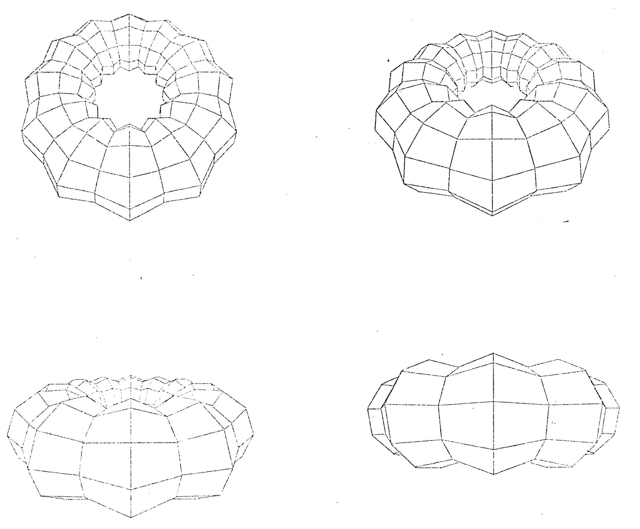
The surface is defined by three two-dimensional arrays X, Y and Z. As these arrays can take on any values, it is easy to define a surface where f(x,y) is no longer restricted to be a single-valued function.
In this example, a torus is defined with 24 segments around the larger radius and 11 around the smaller. The torus is defined so that the start and end points coincide, thus producing a closed surface.
GSURF initialises the surface to be situated around the origin. The first call of CTRAN moves the object away from the viewer so that the whole surface can be seen.
MASTER GSRF
C DISPLAY OF A TORUS USING GSURF
      COMMON/FREE/IFREE(2,23000)
      COMMON/BUCKY/ IB(512)
      DIMENSION X(12,25),Y(12,25),Z(12,25)
      CALL INFREE(23000,512)
C THE RADIUS OF THE CROSS SECTION WILL ALTERNATE
      R1=20.
      R2=25.
C THE RADIUS OF TORII WILL STAY FIXED
      R3=50.
C THERE WILL BE 11 DIVISIONS AROUND THE CROSS SECTION
      IC=l2
      TS==360./FLOAT(IC-1)
C THERE WILL BE 11 DIVISIONS AROUND THE OUTSIDE
      IO=25
      PS=360./FLOAT(IO-1)
      PD=-PS
      K=0
      DO 1 J= 1,10
      PD=PD+PS
      P=PD*3.1415926536/180.
      TD=-TS
C ALTERNATE THE RADIUS
      IF (K .EQ. 0) GOTO 10
      K=0
      R=R1
      GOTO 20
   10 CONTINUE
      K=1
      R==R2
   20 CONTINUE
      DO 1 I=1,IC
      TD=TD+TS T=TD*3.1415926536/180.
C GET THE COORDINATES
      X(I,J)=(R*SIN(T)+R3)*SIN(P)
      Y(I,J)=R*COS(T)
      Z(I,J)= (R*SIN(T)+R3)*COS(P)
    1 CONTINUE
      CALL FRHCM
      CALL ADVFLM
      CALL LIMITS (-10.,-10.,512.,512.,1.,1.)
      CALL GSURFI (X,1,12,1,Y,1,25,1,Z,12)
      CALL CTRAN(0.,0.,120.)
      DO 80 I=1,4
      CALL GSURFD (X,1,12,1,Y,1,25,1,Z,12,1,90)
      CALL ADVFLM
      CALL CTRAN (0.,0.,-120.)
      CALL CXROT(20.0)
      CALL CTRAN(0.,0.,120.)
   80 CONTINUE
      CALL ENDSPR
      CALL EXIT
      END
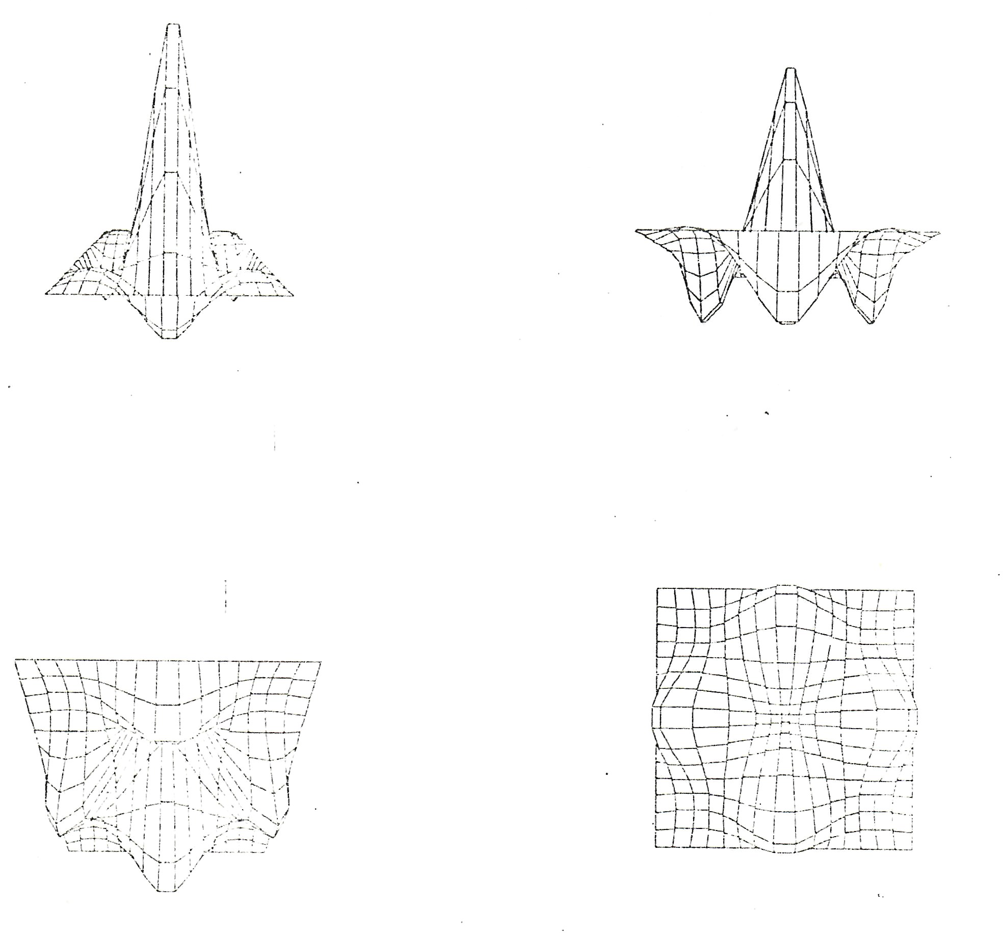
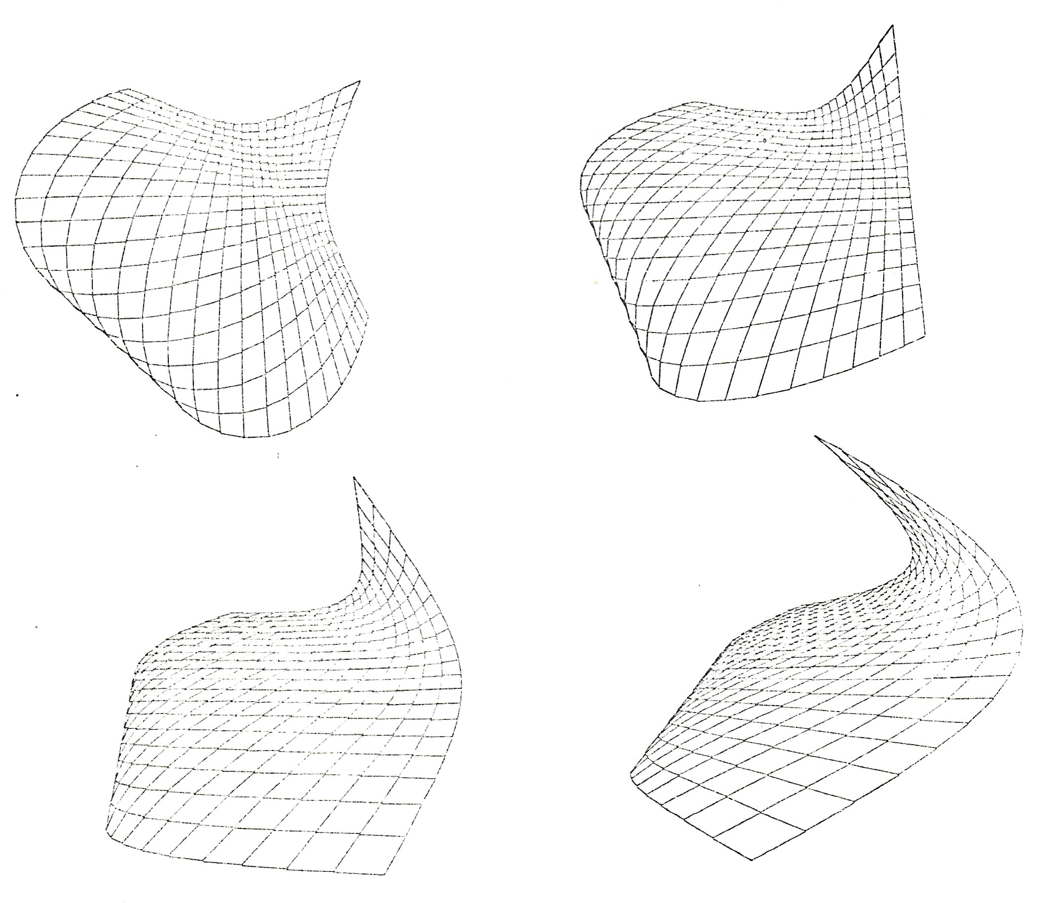
This second example of using GSURF, illustrates how it can be used to define simpler surfaces although it is more likely that one of the other routines would be used in this case. The surface is defined on a grid in the x and z direction with:
y = (π - |x|) (π - |y|) cos(x) cos (z)
In this case, it is only necessary to move the surface back 10 units to get a reasonable view. This distance depends on the coordinates of the surface. It must be at least half the length of the surface in the z-direction to ensure that the complete surface is in front of the viewer. The extra amount needed will depend on the size of the surface in the x and y direction.
      MASTER SINE
      COMMON/FREE/IFREE(2,23000)
      COHMON/BUCKY/IB(512)
      DIMENSION X(16,16),Y(16,16),Z(16,16)
      CALL INFREE(23000,512)
      PI==3.14159265
      DELTA=2.*PI/15.
      DO 100 I=1,16
      XX=-PI+FLOAT (I-1)*DELTA
      DO 90 J=l,16
      ZZ==-PI+FLOAT(J-1)*DELTA
      YY==(PI-ABS(XX))*(PI-ABS(ZZ))*COS(XX)*COS(ZZ)
      X(I,J)=XX
      Y(I,J)=YY
      Z(I,J)=ZZ
   90 CONTINUE
  100 CONTINUE
      CALL FRHCM
      CALL ADVFLM
      CALL LIMITS (-10.,-10.,512.,512.,1.,1.)
      CALL GSURF I (X,1,16,1,Y,1,16,1,Z,16)
      CALL CTRAN(0.,0.,10.)
      CALL GSURFD (X,1,16,1,Y,1,16,1,Z,16,1,90)
      CALL ADVFLM
      DO 200 I=1,3
      CALL CTRAN ( 0.,0.,-10.)
      CALL CXROT (30.)
      CALL CTRAN(0.,0.,10.)
      CALL GSURFD (X,1,16,1,Y,1,16,1,Z,16,1,90)
      CALL ADVFLM
  200 CONTINUE
      CALL ENDSPR
      EXIT
      END
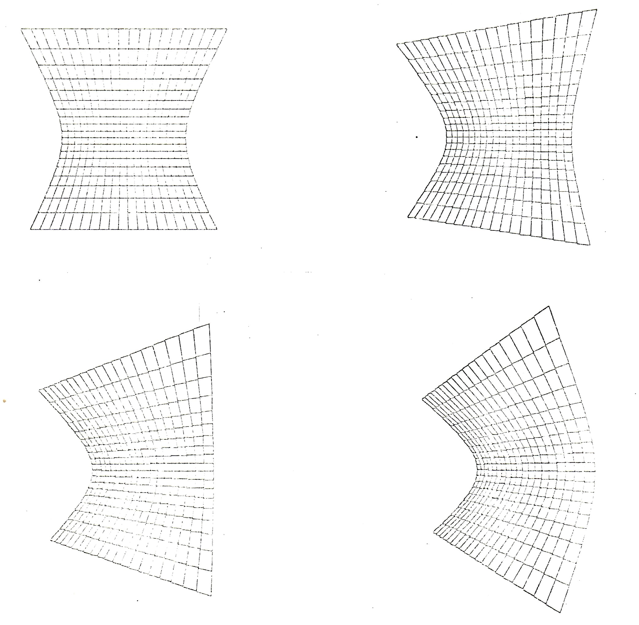
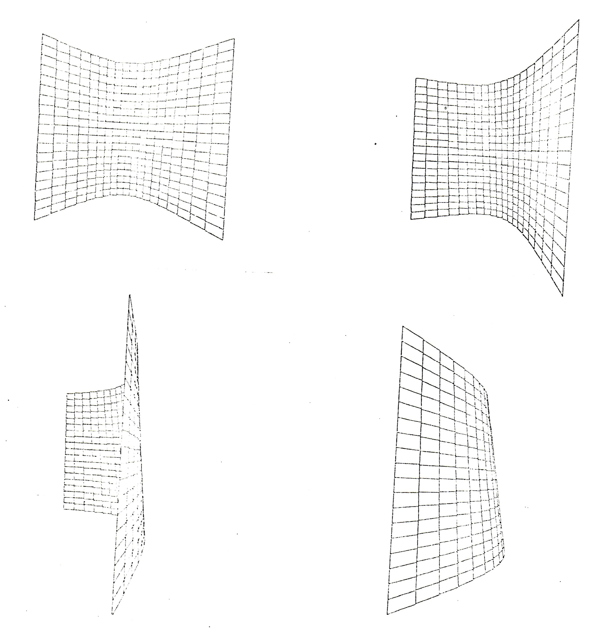
This routine expects the surface to be defined on an equi-spaced grid in the x and y directions with the z coordinates given in the array Z. In this example, the x and y coordinates are defined as going from 1 to 20 in increments of 1. The z values are given by:
z = 10 sin (πy/20)
The surface is a cylinder which is being rotated about the y axis.
      MASTER ESRF
      COMMON/FREE/IFREE(2,23000)
      COMMON/BUCKY/IB(512)
      DIMENSION Z(20,20)
      CALL INFREE (23000,512)
      DO 30 I=1,20
      DO 20 J=1,20
      Z(J,I)= 10.*SIN(FLOAT(I)*3.1415926/20.)
   20 CONTINUE
   30 CONTINUE
      CALL FRHCM
      CALL ADVFLM
      CALL LIMITS(-10.,-10.,512.,512.,1.,1.)
      CALL ESURFI (1,20,1,1,20,1,Z,20)
      CALL CTRAN (0.,0.,20.)
      CALL E SURFD (1,20,1,1,20,1,Z,1,90.)
      CALL ADVFLM
      DO 50 I=1,3
      CALL CTRAN(0.,0.,-20.)
      CALL CYROT (15.)
      CALL CTRAN (0.,0.,20.)
      CALL ESURFD (1,20,1,1,20,1,Z,1,90.)
      CALL ADVFLM
   50 CONTINUE
      CALL ENDSPR
      CALL EZIT
      END
This routine allows the surface to be defined as a function of the form:
z = f(x,y)
FSURF will call the function at each of the nodal points on the surface where x and y range between the parameters passed over to the subroutine. In this example, both x and y range from -10 to 10 in 20 intervals. The surface is defined as:
z = 10 sin (π(x+y)/20)
The surface is rotated about both the x and y axis between each view.
      MASTER FSRF
      COMMON/FREE/IFREE(2,23000)
      COMHON/BUCKY/IB(512)
      EXTERNAL FXY
      CALL INFREE(23000,512)
      CALL FRHCM
      CALL ADVFLM
      CALL LIMITS (-10.,-10.,512.,512.,1.,1.)
      CALL FSURFI(-10.,10.,20.,-10.,10.,20.,FXY)
      CALL CTRAN(0.,0.,20.)
      CALL FSURFD(-10.,10.,20.,-10.,10.,20.,FXY,1, 90.)
      CALL ADVFLM
      DO 10 I=1,3
      CALL CTRAN(0.,0.,-20.)
      CALL CYROT(30.)
      CALL CXROT(7.)
      CALL CTRAN( 0.,0.,20.)
      CALL FSURFD (-10.,10.,20.,-10.,10.,20.,FXY,1, 90.)
      CALL ADVFLM
   10 CONTINUE
      CALL ENDSPR
      CALL EXIT
      END
      FUNCTION FXY(X,Y)
      FXY=1.0*sIN((X+Y)*3.1415926/20.)
      RETURN
      END
RSRF defines a rectangular grid by the coordinates contained in two one-dimensional arrays. The z values are defined in a two-dimensional array.
In this example, the x and. y values are defined as going from -10 to 9 in increments of 1. The z values are defined as:
z = 10 sin(π(x+11)/20) * (49-y)/60
      MASTER RSRF
      COMMON/FREE/IFREE(2,23000)
      COMMON/BUCKY/IB(512)
      DIMENSION X(20), Y(20), Z(20,20)
      CALL INFREE(23000,512)
      DO 10 I= 1,20
      X(I)=FLOAT(I)-11.
      Y(I)=FLOAT(I)-11.
   10 CONTINUE
      DO 30 I=1,20
      DO 20 J=1,20
      Z(I,J) = 10.*SIN(FLOAT(I)*3.14.15926/20.)*(60.-FLOAT(J))/60.
   20 CONTINUE
   30 CONTINUE
      CALL FRHCM
      CALL ADVFLM
      CALL LIMITS ( -10.,-10.,512.,512.,1.,1.)
      CALL RSURFI(X,1,20,1,Y,1,20,1,Z,20)
      CALL CTRAN(0.,0.,20.)
      CALL RSURFD (X,1,20,1,Y,1,20,1,Z,20,1,90.)
      CALL ADVFLM
      DO 50 I=1,3
      CALL CTRAN(0.,0.,-20.)
      CALL CYROT (30.)
      CALL CTRAN(0.,0.,20.)
      CALL RSURFD (X,1,20,1,Y,1,20,1,Z,20,1,90.)
      CALL ADVFLM
   50 CONTINUE
      CALL ENDSPR
      CALL EXIT
      END
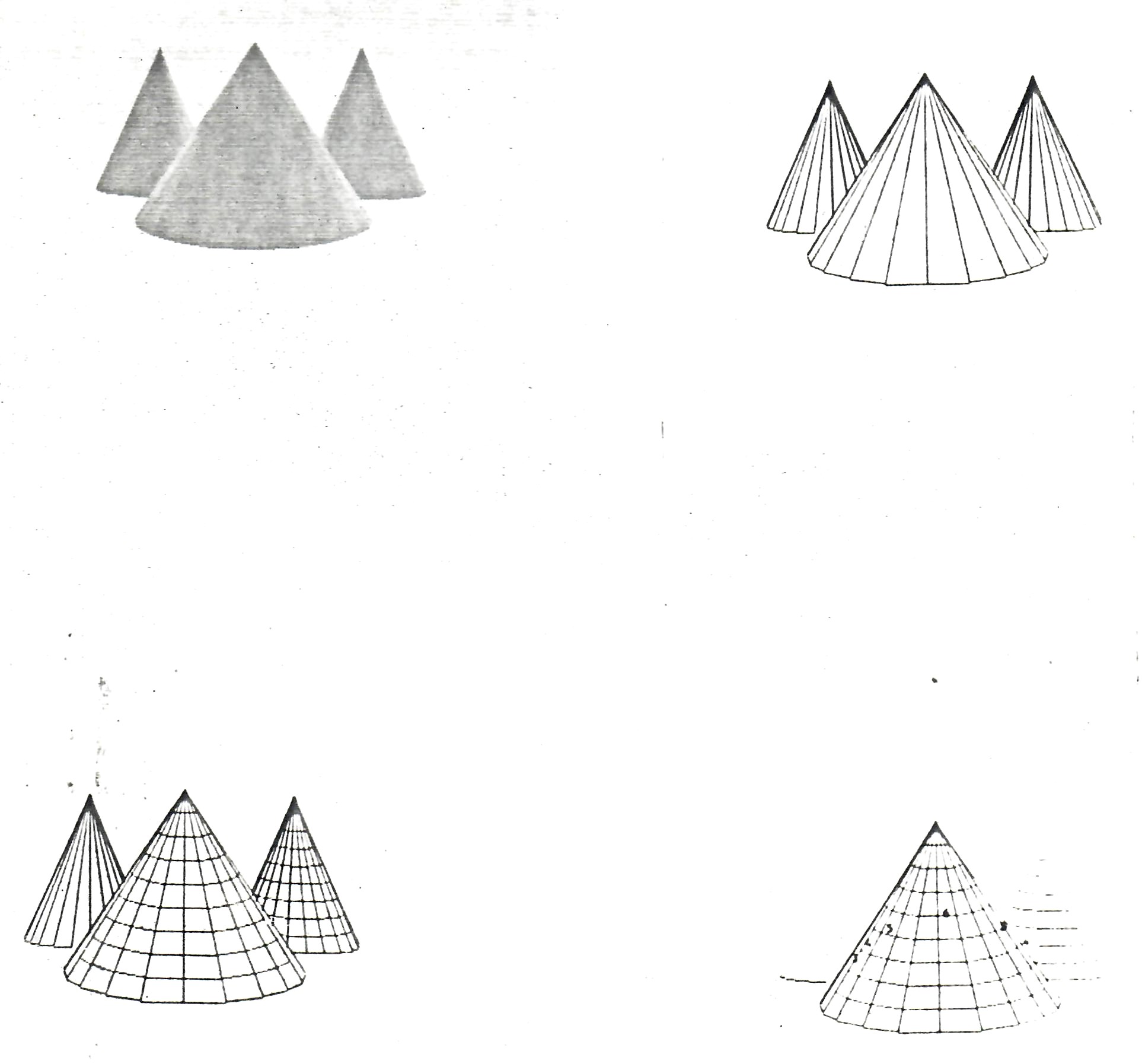
The low-level routine POLCLP allows the user to define the individual polygons making up the objects to be displayed. In this example, the subroutine PYRMID defines a pyramid with the orientation, size and number of sides specified by the user.
In the example, three pyramids are defined. The first does not have shared edges while the third will not have contour bands.
The objects are displayed in a. number of ways to show the various possibilities. The last view indicates that only the bottom of the pyramid is an unshared edge.
      MASTER PYRA
C THIS IS AN EXAMPLE PROGRAH DEMONSTRATING HOW
C YOU CAN USE SEVERAL FEATURES OF THE ALGORITHM IN
C DISPLAYING THREE DINENSIONAL OBJECTS
      COMMON/FREE/IFREE (2,9000)
      COMMON/POLDAT/ICNT,NTERNL,X (12),Y(12),Z(12),S (12) ,
     1KOL(12),CON(12),ISHR(12)
      COMMON/BUCKY/IB(5l2),
      COMMON/QFORIO/CONTRS,IDVICE,IBAD,SHOSHR,LBLSPC
      COMMON/CONLEV/CONHI,CONLO,NCONLV,CLEVEL(10)
      COMMON/ZRANGE/ZMIN,ZMAX
      COMMON/INTENS/IHI,ILO,IBACK,IFRAMX,IFRAMY
      LOGICAL NTERNL,ISHR,CONTRS,IBAD,SHOSHR
C SPECIFY THE MAXIMUM VALUES
      CALL INFREE (9000,512)
C JUMP IF WE GET AN ERROR
      IF(IBAD) GOTO 5
C ESTABLISH THE RESOLUTION
      IFRAMX=512
      IFRAMY=512
      IHI=31
      IL0=8
      IBACK=4
C SET THE RANGE OF Z DATA FOR CLIPPING
      ZMIN=15.8
      ZMAX=44.0
C DETERMINE CONTOUR LEVELS TO BE PLOTTED
      NCONLV=10
      CONLO=2.
      CONHI=10.
      DO 1 I=1,NCONLV
      CLEVEL(I)=I
    1 CONTINUE
C INITIALISE THE POLYGON CLIPPER
      CALL INTCLP
C JUMP IF WE GET AN ERROR
      IF( IBAD) GOTO 5
      CONTRS=.TRUE.
      KOL(1)=0
      KOL(2)=0
      KOL(3)=0
      CALL PYRMID(0.0,6.0,26.0,-6.0,8.0,45.0,24,.FALSE.,.TRUE.)
      CALL PYRMID(10.5,8.0,36.5,-6.0,6.0,40.0,24,.TRUE.,.TRUE.)
      CALL PYRMID(-9.5,8.0,37.5,-6.0,6.0,30.0,24,.FALSE.,.FALSE.)
C INITIALISE THE DISPLAY ROUTINES FOR GRAPHICS
      CALL FRHCM
      CALL LIMITS (-10.,-10.,512.,512.,1.,1.)
      CALL ADVFLM
C DISPLAY THE PICTURE SHOWING ALL TRIANGLES
      SHOSHR=.FALSE.
      CONTRS=.FALSE.
C
C THIS TRIES SHADING
C
      IDVICE=-1
      CALL HIDDEN
      CALL ADVFLHM
C LINES
      IDVICE=1
      SHOSHR=.TRUE.
      CONTRS=.FALSE.
      CALL HIDDEN
      CALL ADVFLM
C LINES AND CONTOURS BUT NO LABELS
      IDVICE=1
      SHOSHR=.TRUE.
      CONTRS=.TRUE.
      LBLSPC=1000
      CALL HIDDEN
      CALL ADVFLM
C CONTOURS BUT NO SHARED EDGES AND WITH LABELS
      IDVICE=I
      SHOSHR=.FALSE.
      CONTRS=.TRUE.
      LBLSPC=10
      CALL HIDDEN
      CALL ADVFLM
      CALL ENDSPR
    5 CALL EXIT.
      END
      SUBROUTINE PYRMID (XTOP,YTOP,ZTOP,YBS,RAD,TH,N,SHRD,CNTR)
C
      LOGICAL SHRD,CNTR
      COMMON/POLDAT/ICNT,NTERNL,X(12),Y(12),Z(12),S(12),
     1IKOL(12),CON(12),ISHR(12)
      LOGICAL NTERNL, ISHR
C PRODUCES A PYRAMID WHOSE APEX IS AT XTOP,YTOP,ZTOP
C THE Y DIRECTION IS THE HEIGHT OF THE POLYGON
C THE Y VALUE AT THE BASE IS YBS
C THE RADIUS AT THE BASE IS RAD
C THE POLYGON HAS N SIDES WITH THE FIRST
C SIDE STARTING AT TH DEGREES FROM X AXIS
C IF CNTR IS TRUE 10 CONTOUR LEVELS WILL BE DEFINED
C WITH HIGHEST AT APEX
C IF SHRD IS TRUE THE EDGES WILL BE MARKED AS SHARED
C
C
      ICNT=3
      NTERNL=.FALSE.
      X(1)=XTOP
      Y(1)=YTOP
      Z(1)=ZTOP
      RPI=3.1415926/180.0
      X(2)=XTOP+RAD*COS(RPI*TH)
      Z(2)=ZTOP+RAD*SIN(RPI*TH)
      Y(2)=YBS
      Y(3)=YBS
      IF(CNTR) GOTO 10
      CON(1)=-1.
      CON(2)=-1.
      CON(3)=-1.
      GOTO 20
   10 CONTINUE
      CON(1)=10.
      CON(2)=1.
      CON(3)=1.
   20 CONTINUE
      ISHR(1)=SHRD
      ISHR(2)=SHRD
      ISHR(3)=SHRD
      T=TH
      DO 50 I=1,N
      X(3)=X(2)
      Z(3)=Z(2)
      T=T-360./FLOAT(N)
      R=T*RPI
      X(2)=XTOP+RAD*COS(R)
      Z(2)=ZTOP+RAD*SIN(R)
      CALL POLCLP
   50 CONTINUE
      RETURN
      END